
Marcus Chatfield
Introduction
Whether it is in slope stability or roof support, the miner needs to be able to assess ground conditions effectively. Boreholes are drilled in order to examine the rock mass. Core samples are taken and, for the most part, offer a measure of intact rock strength as well as the character, frequency and orientation of discontinuities. From this information some form of rock mass rating might be attempted.
Since the borehole has been drilled, there might be a benefit from running a couple of wireline log measurements. The televiewer is an obvious choice due to its superior orientation but all wireline logs offer three big advantages; they are objective, there are no gaps and they are vertically precise; a log is one event. The destructive measurement of pieces of drill-core comprises multiple events. It is not precise and there may be core loss; gaps in the data set. Selection of core pieces is subjective
The strength and elasticity of the underlying rock matrix (IRS) may be estimated using a full-waveform sonic sonde. The combination of laboratory and wireline techniques is so powerful that it demands some consideration by the geotechnical engineer. Following is a review of the sonic log and its derived measurements
Principles of Sonic Logs
The various sonic transit time logs available to the geologist and geotechnical engineer should be both precise and accurate. There are important empirical relationships between these reliable sonic logs and rock strength and elasticity. It is important to understand why the logs are normally accurate and what can compromise log quality.
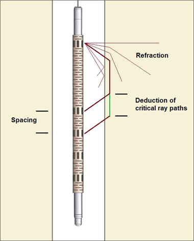
The compression wave transit time measurement (Figure 1) is based on the deduction of the travel time of a refracted wave from transmitter to receiver 1 (the closest receiver) from the travel time from transmitter to receiver 2 (20cm further away).
If the spacing of the transducers is 20 centimetres, the result is a log of the transit time in micro-seconds through 20 cm of rock. If that time is multiplied by 5, we get a transit time log in micro-seconds per metre. All variables such as ray path, fluid velocity and borehole diameter are deducted out. The log does not require calibration as its response depends entirely on an accurate clock (assumed) and a fixed tool geometry (sometimes requiring verification by multiple log overlay).
What can go wrong?
Two variables affect the accuracy of the sonic log in adverse borehole conditions. These are signal amplitude and ray path. A low signal amplitude makes first arrival discrimination difficult and borehole caving extends the measured critical path, particularly for the shorter transducer spacings.
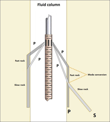
In hard/fast rocks (Figure 2), the first arrival amplitude is naturally low due to high formation elasticity. These first breaks can be difficult to discriminate.
These problems may be overcome during data processing but logger’s client might be disappointed to learn that the monopole sonic used in mineral logging cannot measure the shear wave transit time in slow formations.
This is the significant limitation of the (Mineral) Monopole Full Waveform Sonic tool.
If the shear wave velocity in the formation is slower than the compression wave velocity of the fluid in the borehole column, the transmitted signal will be refracted away from the borehole and cannot be measured.
Unfortunately, there is no perfectly reliable way around this problem (in oilfield logging they use the very sophisticated dipole sonic tool). The only option is to use some empirically-based formula, using
P-wave sonic and density data, to estimate the shear wave transit time. This technique is well tried and there are many formulae which, at least, retain precision in the log.
The movement of the sonde along the borehole, particularly an angled borehole, sometimes causes “road noise” that is picked up by the receivers. This will make first-arrival discrimination difficult in hard rock data. The transmitting and receiving transducers degrade over time making them less sensitive and reducing the amplitude of the log. A comparison of statistics from various transducers and/or various sondes will allow the logger to become familiar with what is normal, in terms of amplitudes at different spacings, and what is low. Signal to noise ratios will be usually be compromised over time.
In the example in Figure 3 all three logs are poor but the far receiver signal (right) has been submerged into the amplified road noise and is hardly visible…time to change the transmitter.
Auto-picking of the first break is important to retain sonic log precision.
The log analyst may use various first-break discrimination techniques but the golden rule is, if you are going to log hard fast formations…take a good sonde and centralise it!
Lack of tool centralisation, especially in large diameter boreholes, results in the signal’s arrival being splurged due to circumferential ray paths having different lengths. Again, the effect is deducted away but good centralisation resulting in a sharper higher peak amplitude will improve discrimination.
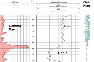
The sonic tool will not operate above the borehole fluid level. Its log will also be adversely affected by gas in the borehole fluid. A poor log caused by gas bubbles (Figure 4) often confuses the logger who thinks there is something wrong with his sonde (he should do a repeat and look for common start depth of the gas ingress).
Gas bubbles travel along the high side of the borehole and the sonde travels along the low side but gas still causes problems to data quality. The only solution, on the basis that the effect is random, is to record multiple runs and stack the data. This works rather better on full waveform data sets where further stacking of waveforms (vertical moving averaging) is possible.
Sonic Transit Time Measurement by Deduction
Some things can go wrong but, in most cases, borehole conditions are conducive to the capture of precise P-wave sonic logs and precision and accuracy are inherent in the system. This is the strength of the sonic log and it is vital if the logs are to be used in geotechnical studies. They are also used for cross-hole correlation and to estimate porosity, flag secondary porosity (in conjunction with density porosity), describe lithology, correct surface seismic records and create synthetic seismograms. Their peak amplitude log is used to evaluate cementation behind casing (CBL or cement bond log).
If the first break is clearly visible, its discrimination is quite straightforward during data processing. It is then necessary to
perform the various deductions (refer to Figure 5), for example:
(T1R2-T1R1)*5 (T1R3-T1R1)*2.5 (T1R4-T1R1)*1.667
Some depth alignment may be necessary.
Borehole compensation is not normally required in mineral logging but it is available from specialised dual transmitter tools and, rather cleverly, by mathematical comparison of two deductions of similar resolution.
If the borehole is caved or fractured, there may be some overstatement of transit time due to a longer ray path or one that includes water in open fractures. The shorter spaced logs will have a higher resolution, which is desirable, but suffer more from borehole irregularities.
Longer spacing will result in the ray path being deeper in the formation and cause a slightly faster log from (T1R4 – T1R1)*1.667, for instance, because the shorter T1R1 might be affected by near- hole fractures and caving. This effect is not normally significant in cored boreholes.
Log compensation is available if a second transmitter (T2) is present on the sonde (not the norm in mineral logging). In which case, data stacking is available.
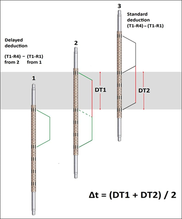
Mathematical compensation of single transmitter data using the delayed deduction of T-R measurements is illustrated in Figure 5.
A stack of two separate measurements is achieved by deducting the remembered green ray path time in position 1 from T1-R4 in position 2…leaving the first red measurement DT1.
The result is compared with the standard deduction of T1-R1 from T1-R4 in position 3…which leaves the second red transit time measurement DT2. This can occur real-time as the sonde logs the borehole.
The two logs target the same formation (the grey layer) but are based on different deductions from ray paths covering different sections of borehole. The analyst can then stack or take the shorter of the two transit times. This technique offers a better sonic log if only one transmitter is available.
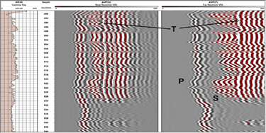
Using the VDL Image
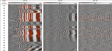
The dual image log in Figure 6 is a really good example of a clean VDL (variable density log) set of images. No road noise is visible. Compression wave (P) and shear wave (S) fronts are clearly defined. Even a third front, the Stoneley (tube) wave (T), can be seen on both images.
Note that when both transit times increase (in slower rock), near to the bottom of the log, the shear wave front disappears.
The Tube Wave is not a refracted wave. It is a surface or interface wave whose path is constrained by the borehole. The tube wave transit time is affected (slowed) by formation permeability. Part of its energy may be reflected back up or
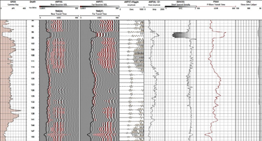
down the borehole wall if it encounters the sharp edge of an open fracture. This causes a chevron pattern on the VDLs (see depth 93-96m in Figure 7).
Some sonic tools (a 3ft – 5ft CBL tool for instance), have just two receivers. First breaks can be picked automatically and deducted, resulting (after correction to the universal lengths of foot or metre) in an objective measurement of P-wave transit time (Figure 7). If there are three or four waveforms logged, a semblance image may be derived from the data (Figure 8).
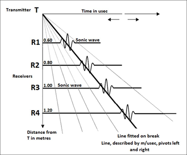
The diagram in Figutre 8 describes a line pivoting at zero time/
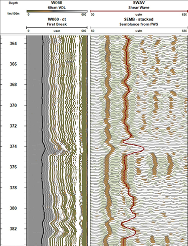
distance (T). The slope of this line is the ratio of time and distance from T. It is therefore described in usec/metre or usec/foot. At each intersection of line and sonic wave trace, in this case there are four waves, a coherence value is calculated and stacked semblance image derived. “It is the ratio of the energy of stacked traces to the sum of the energies of the individual traces within a time window” (WellCAD). The resulting semblance image is used to shift a nearby log curve, provided by the analyst, onto the extremum or highest peak on the semblance waveform.
In the example in Figure 9, a log was drawn by hand to roughly follow the second peak on the semblance image. This was then shifted using the extremum adjustment to follow the peak. Some manual editing was necessary where the peak disappeared.
This is the end-product of the logging operation, a reliable and mostly objective measurement of P and S wave velocity.
The lack of a shear wave log in soft formations may seem to be problematic but that log may be estimated using one of several well-known formulae that employ P-wave sonic and density. Christensen’s equation is one example. The estimation of the shear wave transit time can be adjusted by comparison to the measured shear front where it is visible.
Having generated a good set of P and S waves, the logger can derive some useful geotechnical data.
Engineering parameters
The rock mechanics engineer would like to be able to measure a formation’s propensity to compress, expand and shear when stressed. Because these phenomena are related directly to the formation’s elasticity, it should be possible to use wireline logs of compression (P) wave and shear (S) wave velocity to calculate Poisson’s Ratio and, with density, to calculate some of the various elastic moduli.
- Young’s Modulus – axial stress versus axial strain (stiffness)
- Shear Modulus – propensity to deform under shear stress (rigidity)
- Bulk Modulus – resistance to compression
These are all derived logs of stress versus resulting strain.
Stress is the force acting on the rock mass and strain is the resulting deformation. Usually, a compressing force will result in longitudinal shortening and transverse extension. There may be some shear effect as well. The ratio of strain to strain is called the “strain”. This is the amount of deformation in length, width or volume compared to the original dimensions. If the stressed object changes in length by 10% its deformation is 0.1 strains.
Note that Poisson’s Ratio is the ratio between the extents of the strain caused by the sonic wave’s compressive force (axial) versus the amount of strain caused by its shear force (lateral). The strain is reflected in the ratio of the two velocities; VP/Vs.
These strains occur at the molecular level. The moduli describe the inherent elastic properties of the formation based on its
chemistry. They do not necessarily describe the elasticity of the rock mass as a whole. The rock engineer will normally refer to milli-strains whereas the effect of a sonic wave on the formation is in the order of a few micro-strains. This results in a problem…
Dynamic measurements of elasticity tend to overstate compared to static measurements (in the laboratory) and the “truth” (in the mine).
The formation includes rock matrix and porosity; primary pore spaces or secondary fractures. Even igneous rocks include micro-pores and micro-fractures. These tiny spaces will elastically deform under stress. The extent of this deformation will certainly depend on the rock’s inherent elastic properties, its stiffness, but also on the overburden pressure , the size and shape of the pore spaces, and the hydraulic pressure (pore pressure) endured by the fluids within them. It seems unlikely that the tiny stresses imparted by sonic waves would be enough to distort these relatively large components of the overall rock mass, so it appears to be stiffer than it is.
Having said that, there seems to be some real value in having a baseline or matrix-level measurement of elastic properties. The added effect of spaces within the rock fabric is difficult to quantify but it will depend, to a large extent, on the inherent rock matrix stiffness. Qualitative use of the dynamic logs of elasticity (low, medium, high etc.) appears to be valid, particularly in tight formations. A typical variance from static values is about +15%.
Intact Rock Strength
Another geotechnical objective is a continuous high resolution log of intact rock strength (IRS) in terms of uniaxial (and unconfined) compressive strength (UCS) calibrated in MPa or PSI units.
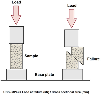
The laboratory technician measures rock strength by applying stress to a piece of drill core in one direction (uniaxially) until it fails (Figure 10).

The unconfined compressive strength of a core sample is calculated by dividing the stress or compressive load recorded at the moment of failure by the sample’s cross-sectional area. UCS log units are, usually, PSI or MPa.
- 1 PSI = load in lbs. / area in square inches
- 1MPa = load in Newtons / area in square mm
Since the advice is to measure and average at least three samples from a core stick, the effective resolution of the measurement is not normally better than about a foot.
This is similar to the wireline log’s resolution but there is a problem. In broken, weathered or otherwise weakened rocks, the laboratory technician will struggle to find undamaged
core samples of sufficient length to validate the test or to be representative of the formation. There will be gaps in the data where it is most needed; in the weaker zones.
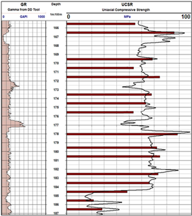
Where laboratory UCS data are available, they should offer a reference with which to calibrate wireline logs if some form of empirical relationship exists. McNally, 1990 in “The Prediction of Geotechnical Rock Properties from Sonic and Neutron Logs” (1990) got the ball rolling in empirical analysis by describing a relationship between sonic transit time logs and UCS measurements in Australian coal basin sediments (Figure 11). There is scatter in the empirical correlation. A sample of the derived UCSR log and the calibration UVS points an core taken along the borehole is shown in Figure 12.
The empirical relationship was strongest in clean sandstones, poor in clay-rich formations and the study did not extend to hard rock transit times. Nevertheless, McNally’s efforts represented a breakthrough and offered conversion of hundreds of very precise sonic logs.
- UCSA(MPa)=1000exp((-0.035)*{DT})
Where DT is the sonic transit time log in micro-seconds per foot.
It soon became clear that tighter and more valid relationships could be found by limiting data to individual geological settings. A site-specific empirical relationship converting sonic or sonic and density logs results in a continuous precise log that is laid on top of discrete imprecise laboratory data…each log supports the other.
Conclusion
P and S wave sonic logs require some processing effort in order to retain precision and objectivity.
Since no calibration is necessary, the sonic log lends itself to geotechnical applications, where precision, accuracy and objectivity are important.
Rock strength and elasticity estimation is valid as long as the limitations of the techniques are understood.
References
McNally, G.H., 1990 – The prediction of geotechnical rock properties from sonic and neutron logs. Exploration Geophysics 21, 65-71.
ALT Sarl, 2020. – WellCAD 5.4 brochure.
Wireline Workshop Bulletin issues – 4 (March 2014), 16 (March 2016), 28 (March 2018), 28 (May 2018) and 30 (July 2018). http:// www.wirelineworkshop.com/bulletin.html Weatherford, 2006 – Weatherford Mineral Logging catalogue.
Author Bio

Marcus Chatfield
Owner/Manager Wireline Workshop (Pty)
Ltd of South Africa Plot 232, Pelindaba Road Broederstroom North West Province Republic of South Africa
After five years Marcus became manager of what had become Reeves Wireline Services in South Africa and lead the company through a hectic gold boom, which involved logging very deep boreholes with lots of tools. Deepest borehole logged; 5115 metres. Marcus has worked throughout Africa, Chile, Alaska, Europe, Colombia, USA and UK.
Reeves were bought out in 2004 by Precision Drilling then Weatherford took over and, after a very interesting two years with that company, Marcus set up his own enterprise, Wireline Workshop.
Wireline Workshop Provides mineral logging services throughout the region.
After a poor start, Marcus fell on his feet when he joined BPB Instruments in 1980 as a borehole logging assistant. His job was to run forward when a sonde appeared and clean it!
This is a story of a practical hands on manager/logger who still logs boreholes today. He is self-taught and thoroughly enjoys the business. The second edition of his book is due in January and the bimonthly bulletin is distributed to over 6,000 geologists and loggers worldwide