
Abstract
Magnetic surveys have been widely used in mineral exploration for many decades as a mean of obtaining structural and geological information. Airborne magnetic surveys are quite common providing large areal coverage over a short span of time, but require complex logistics involving aircraft (helicopter or fixed wing), fuel licenses and transportation, as well as complex health and safety concerns. An alternative is to do ground magnetometer surveys but field production is not as efficient as with airborne surveys. The necessity to obtain high resolution magnetic information over intermediate-size areas that could be considered too large for ground work production and too small to justify aircraft logistics, has opened the possibility of using drones as the magnetic sensor carriers.

Introduction and Survey Area
Freeport-McMoRan (FMI) is one of the senior mining corporations in the world leading the use of unmanned aerial vehicle (UAV) magnetometer surveys projects. In January 2020, and as part of their exploration programs, FMI commissioned Arce Geofísicos to conduct a survey for their Rapsodia project in Southern Perú.
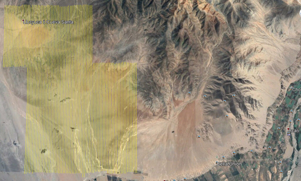
The survey was conducted for FMI’s Peruvian subsidiary, Exploraciones Antakana S.A.C. and the area is located next to the city of Bella Unión in Arequipa, approximately 570 kilometers South of Lima, accessible through the Panamerican Highway.
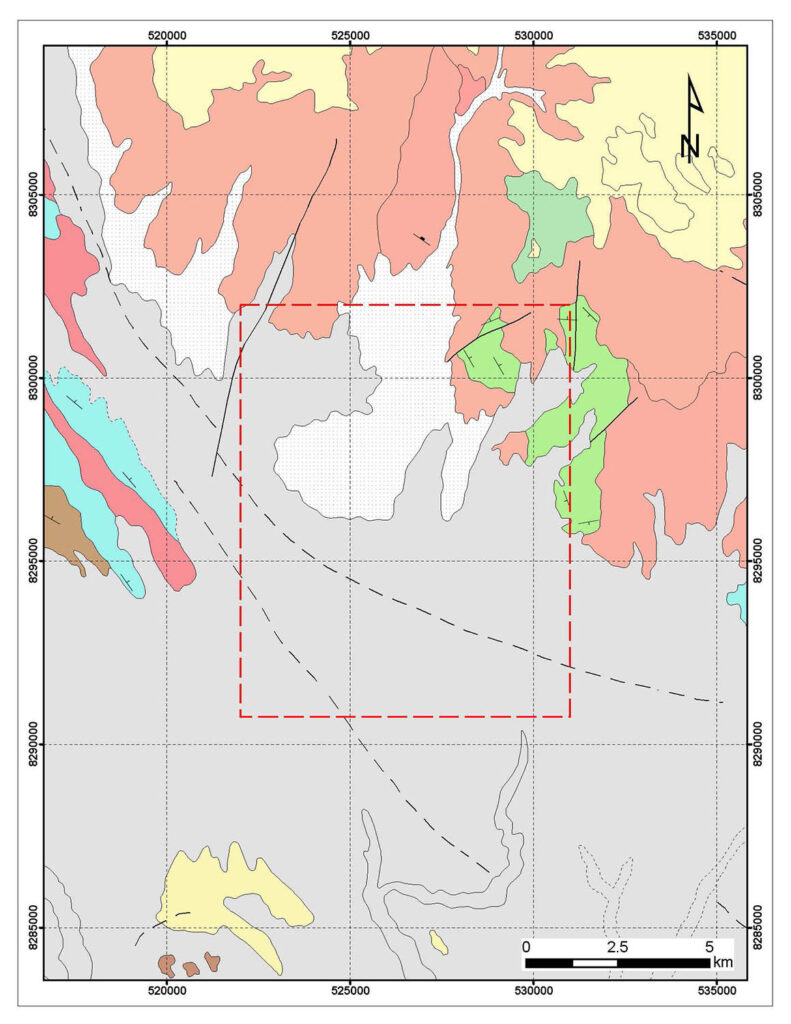
Rapsodia is located in the Peruvian Coastal Batholith region. The Cretaceous age batholith consists of the Acai diorite intruding into the early Cretaceous Huallhuani formation, composed of quartz sandstones with interbedded grey limolites.
Survey design and flight parameters
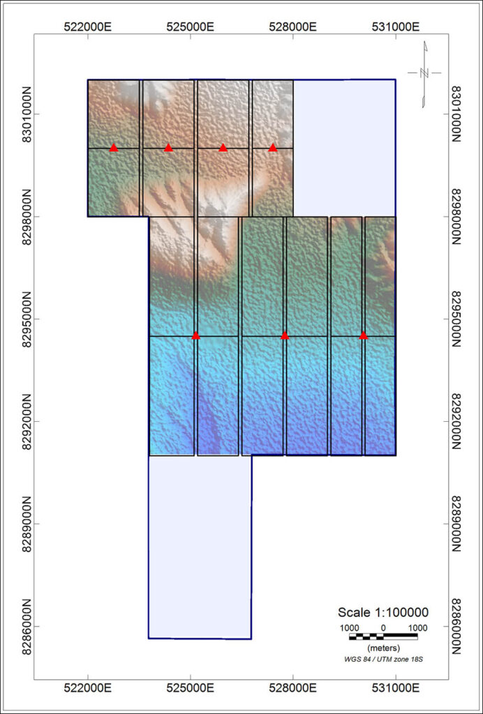
The survey consisted of an original plan of 916 line kilometers of North-South profiles with a line separation of 100 meters, of which 832 kilometers was completed. The area was split multiple blocks with 2 to 3 kilometers length, considering that the maximum flying time was around 25 minutes and between 10 and 15 kilometers per flight, depending of the terrain, weather and battery performance. Figure 3 shows the blocks and takeoff and landing base locations used at the project.
The survey was performed over 18 days of production, considering 4 additional days of mobilization/demobilization and travel time from Lima. The crew consisted of 1 geophysicist and drone pilot, 1 field geophysicist QC, 1 geophysicist operator, 4 local helpers and 1 senior geophysicist based in Lima.
The daily production was:
Minimum: 9.12km per day
Maximum: 95.22 km per day
Average: 46.26 km per day
Mission planning and monitoring
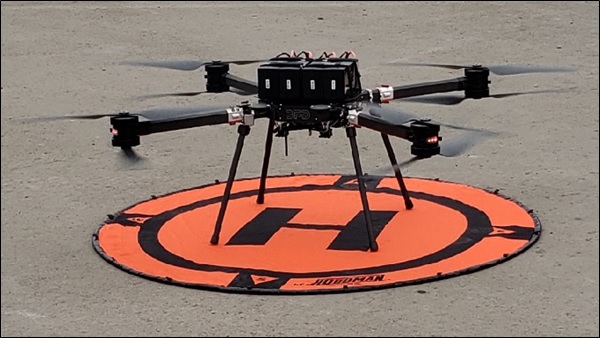
The UAV used was a quadricopter manufactured and customized by BFD Systems 1400-SE8, powered by 4 LiPo batteries of 22000 mA/h capacity each, with a flight computer on board from Ardupilot (Cube) and 8 weather sealed motors, which provide up to 26 minutes endurance flight time, using a maximum payload of 12.25 kg in normal conditions (Figure 4A). In addition, the copter has a laser altimeter with a maximum measuring height of 100m.
A high precision potassium-vapor GEM Systems magnetometer was used. This sensor was part of the GEM Airbird towing system (Figure 4B). This sensor offers very high sensitivity with small heading error with an absolute accuracy of 0.1nT and sampling rate of 10Hz. The Airbird ensured a smooth operation and high quality readings due to its mechanical stability and aerodynamics.
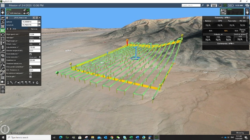
The survey area was provided by the client to prepare the survey plan and flight lines. Based on the terrain access and station locations, the survey area was split into several polygon zones, exported to kml and used to create the flight mission plan using the UgCS software version 3.4.609. The following parameters were considered:
Line separation: 100m
Flight height: 40m ~ 50m ground clearance.
Extended distance outside each block: 250m to achieve 500m overlap.
UgCS software allows mission planning in terrain-following mode, enabling a very-low- flying vehicle to automatically maintain a relatively constant altitude above ground level, ideal for this type of surveys. The accuracy of the default SRTM database of UgCS varies, therefore, the software allows import a detailed DTM (Digital Terrain Model) for precise and safe flight altitude control. For the project a DTM with 10m resolution was purchased from Intermap (https://www.intermap.com/nextmap).
It is critical to have a high resolution DTM prior to commencing the UAV magnetic survey, particularly in areas with difficult topography, to increase reliability in terrain following, considering that lower ground clearance yields better magnetic field sensitivity and resolution. The flight height programmed in the survey varied from 40 to 50 meters above ground, considering the tow cable’s length of 10 meters and uneven topography in specific areas as well as a desirable flight speed of 15 m/s.
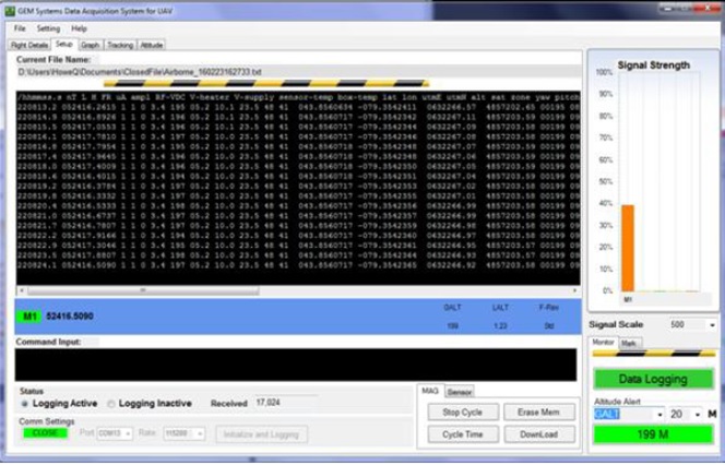
Real time magnetic measurements monitoring was performed with the Airbird ground control software, which provided not only sensor readings and field strength, but also laser altimeter ground clearance.
Acquisition and Data Processing
Quality Control
Before the start of the survey, Geosoft scripts were generated to make quick quality control and pre-processing of collected data. During daily QC, it became clear that the best time to acquire magnetic data was early in the morning; this is mainly due to the fact that in those hours there is less wind, improving sensor aerodynamics, obtaining cleaner readings. The best hours for flight were from 6 AM to PM (noon).
Right after the copter landed in each sortie, survey data were downloaded from the Airbird using its telemetry communication and imported into Oasis Montaj for QC. The raw data were always maintained in its original form in a channel and all further processing was done in new channels.
There were methods used to handle the field data:
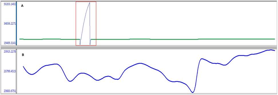
Case 1: Dead-zones. To correct these, a filter was applied over the channel “L” coming from the raw data, which placed dummy values at all rows where the logged value was “0”. These sections or “Dead Zones” of the dataset are caused by the magnetic sensor coming out of signal-locking range, usually due to crosswind and low speed performance. In Figure 7 below, we can see the raw signal (A) with a dead zone, when the sensor was not coupled with the magnetic field (lock parameter L=0) and the signal pre-processing once the unlocked information was filtered and interpolated using the Akima method (B).
As a next step, a fourth difference filter was applied over all data points exceeding the sensor absolute precision specification of 0.1nT, in accordance to the manufacturer’s specifications. The fourth difference filter is widely used in aerial magnetic surveys to identify data noise that exceeded acceptable parameters.
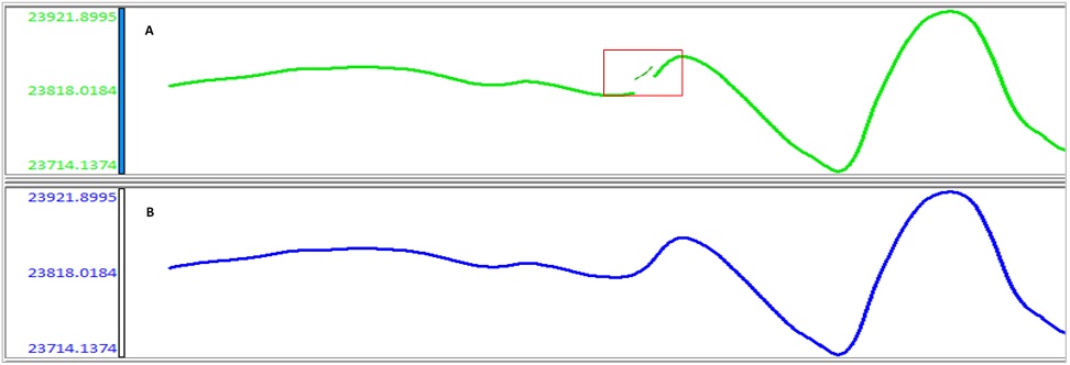
Case 2: Data Jumps. The magnetic data acquired was very clean for most of the survey because the sensor was towed with a 10 meter kevlar cable, far enough from the copter, reducing magnetic noise effects. However, in presence of crosswind and rough topography, the sensor makes sudden movements when climbing up or descending, producing a low speed motion and velocity changes causing instability in the sensor pitch. For this case, a jump constant difference was calculated, and the signal was recovered and interpolated using Akima method when the distance did not exceed more than 100 meters of ground distance, otherwise the line would be repeated under better conditions. Figure 8 shows data jumps with raw and filtered/interpolated signal.
Corrections
Magnetic field readings were compensated by diurnal drift using a GEM GSM-19T base station with a proton precession sensor with GPS incorporated for time synchronization with the Airbird. Daily base station data was cleaned using a non-lineal filter to remove spikes produced by geological noise, geomagnetic storms or sun activity, as part of the daily quality control.
The magnetic heading effect was determined on site by flying a North-South oriented pattern, at a height of 150 meters over terrain. At least one pass on each direction was flown over a recognizable magnetically “flat” feature on the ground to obtain sufficient statistical information to estimate the heading error. A heading effect was considered for lines flown from North to South of -0.331 nT.
A lag test was performed over the data to determine the time difference between the magnetometer readings and the GPS System location in the bird, applying 1 meter back, since that is the distance position between the center of the bird where the GNSS antenna is located and magnetometer sensor position. A negative lag will shift the data forward in time, in this case a lag of -1 fiducial was determined by the average speed channel (10 m/s), and the magnetometer frequency of 10 Hz.
Microleveling
Since tie-lines where not considered from the beginning of the survey, the levelling process was not applied, but a microleveling procedure was used.
Once the data was cleaned and corrected by diurnal, lag and heading correction, levelling problems were noticed along survey lines like data shifts in between lines, caused for the most part by differences in ground clearances in the line overlaps between blocks. This resulted in responses biased to the used line orientation as shown in Figure 9. To correct this, an FFT decorrugation filter was applied to yield a grid that contained the leveling error; a combination of a Butterworth High-Pass filter combined with a Directional Cosine filter was used. The first one, cleaning up the low-frequency noise, and highlighting the high-frequency trends (Rioul et al., 1991), while the second one removing directional noise using the flight line azimuth.
The resulting grid was an error grid with stripes parallel to the line direction. The error value was sampled from the grid and cleaned through a Low Pass filter to separate the high frequency geological signal from the longer wavelength levelling error (Geosoft, 2020). A cutoff wavelength of 1000 fiducials were used (10 times the line separation: 10 x 100m = 1000 fiducials). Once the error was filtered, this value was subtracted from the original grid and a leveled grid was obtained as shown in Figure 9B.
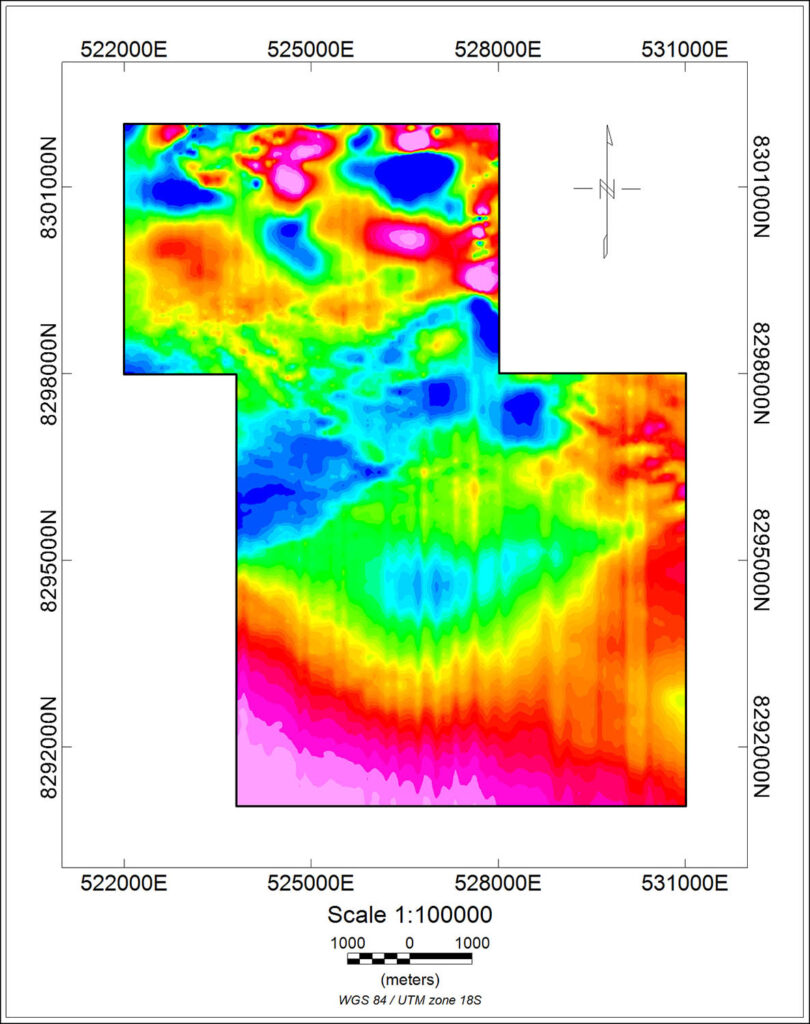
Reduction to the magnetic pole for low latitudes (RTPLL)
The reduction to the pole is a geophysical tool frequently used to estimate and simplify location, intensity and symmetry of magnetic anomalies. When a magnetic survey is performed, all magnetic responses are affected by distortions of their shape, size and location caused by survey location within magnetic latitudes, making this procedure an important step to understand results. Moreover, a standard Reduction to the Pole (RTP) procedure commonly yields mathematical artifacts when the data was obtained close to the magnetic Equator (+/- 30 degrees of magnetic latitude). In this case, an RTPLL was performed (Figure 10) considering an IGRF intensity of 23992.2 nT, a regional field inclination of -7.3 degrees and a declination of -3.1 degrees.
The strong magnetic anomalies in the Northern area may be attributed to the presence of Coastal Batholith rocks and the high zone in the center of the map could be interpreted as the influence of the Cerro Batidero in contrast with the quaternary colluvial type deposits.
The South zone is magnetically flat, and characterized by long wavelength responses attributed to the possible geological configuration of the basement and the overlying sedimentary cover.
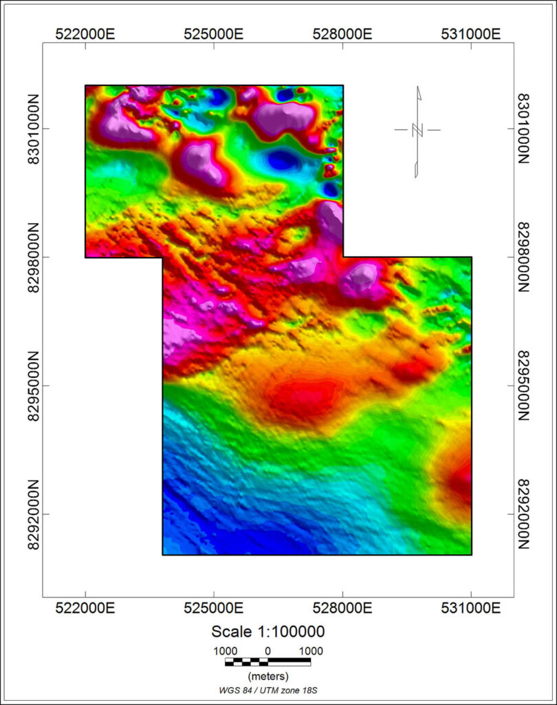
Analytic Signal of Vertical Integration (ASVI)
The ASVI can be defined as the square root of the sum of the squares of the derivates in the X, Y and Z directions of the Vertical Integration of the TMI. The objective of this filter is to better define the edges of magnetic and non-magnetic bodies that cause the anomalies, and provide a cleaner response than a standard Analytic Signal calculation.
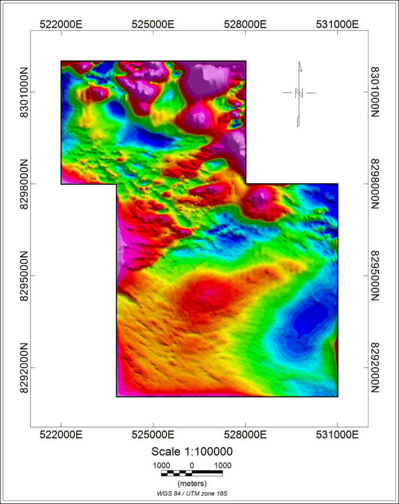
Tilt Derivative (TDR)
The tilt derivative was quite helpful to map shallow responses and structures. This filter has the advantage of enhancing and sharping the magnetic trends yielding geophysical structures.
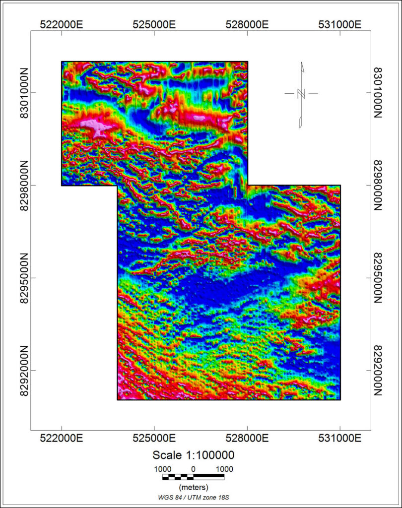
Geophysical Structures
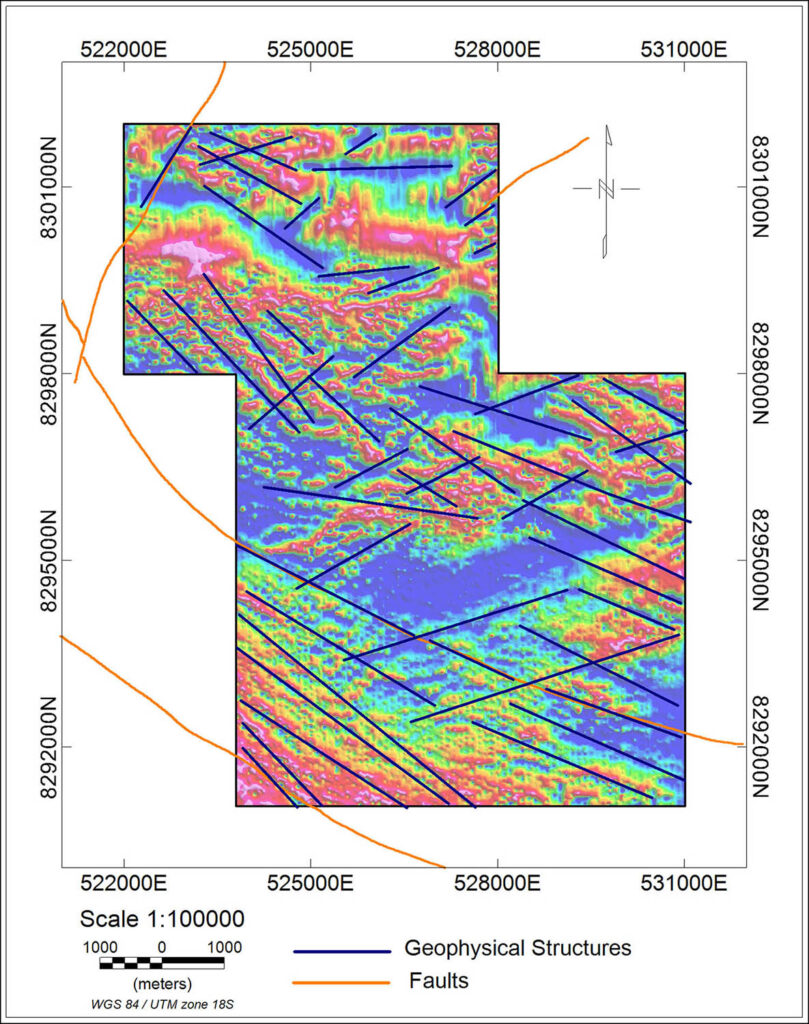
The TDR map was used for geophysical structural interpretation, as its theory indicates that the zero contour line will be located at or very close to the a fault or geological contact. Tracing the zero contour line of the TDR map delineates the subsurface structure of the area and thus drawing possible faults that characterize the area (Esmat E., et al., 2015).
Two fault systems were distinguished in the survey area; the first one with a NE-SW orientation following general Andean regional fault trends, and the second one with a NE-SE orientation. Regional faults presented in orange were downloaded from the Geocatmin system of the INGEMMET (Instituto Geológico, Minero y Metalúrgico of Perú). This public system (https://geocatmin.ingemmet.gob.pe), offers geological and mining information of Peru and served like starting point to identify the rest of geophysical structures (black lines) using the TDR map, as shown in Figure 13.
Magnetic Modelling
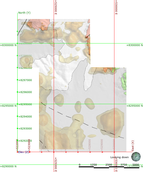
An MVI 3D modelling was performed on the magnetic dataset. One of the main advantages of using an MVI inversion over a standard magnetic susceptibility inversion is its capability of obtaining more realistic results when magnetic remanence is present in the data. This is why MVI inversions are usually easier to interpret with local geology than magnetic susceptibility inversions. An MVI inversion produces for each cell in space, a vector which indicates direction of magnetization and intensity. The inversion results may be seen in Figure 14.
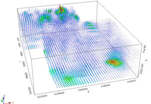
The inversion led some interesting results, which are not easily interpretable from the geological map as most of the area has quaternary sedimentary cover, except on the Northern and Northeastern edges of the survey area. The Huallhuani sandstones in the NE edge have no response in the magnetic inversion and the Acarí batholith shows as a magnetic high that is trending East-West and then South East. High amplitude magnetization responses are seen in the South and South Eastern areas. Magnetic high responses seem to be forming into a circular shape with a magnetic low center located under recent sedimentary cover.
Flight and Survey Safety
When a geophysical survey is carried out, it is of utmost importance to operate under the highest standards of safety for both the crew and geophysical equipment. A UAV survey is not the exception, due to the increased hazards and potential risks associated with the use of an aircraft, particularly in surveys with difficult topography. Some fundamental aspects have to be guaranteed, such as good radio telemetry control range, high-resolution Digital Elevation Model, direct line of sight with the UAV and a good programming system which makes the aircraft properly follow terrain with a safe ground clearance.
On February 22th, 2020, during the ferry part of a flight, a crew member noticed the drone was flying at lower altitude than expected, and when the pilot tried to get control of the UAV though the remote controller, there was no communication between the UAV and both the remote control and base station radios. A note must be made that there is always a small delay when sending an emergency command to a UAV and in this particular case, it would’ve been too late anyway to make the UAV fly higher or return to base. A description of the accident is shown in the Figure 16.
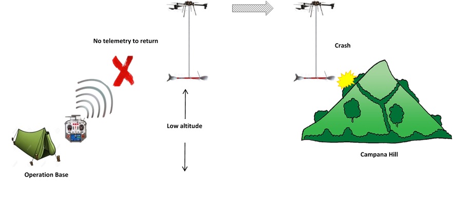
When the causes for the accident were analyzed, the crew noticed that the software did not take into account the DTM for terrain following between the copter homepoint and the beginning of the survey lines, in order to keep ground clearance at a safe level, so the aircraft did not do any terrain draping in this part of the flight, but maintained a constant altitude, resulting in a crash 10 meters before reaching the top of a small hill.
Even though flight programming software allows users to follow terrain using a previously loaded DEM, these do not consider waypoints to modify ground clearance automatically in the area between the base and survey lines. To guarantee a safe flight an additional waypoint path should be programmed manually with enough waypoints from the homepoint to the beginning of the survey line path as well as from the end of the flight to return to the landing base once the flight is complete. This is critical for in a project with difficult topography.
Further issues were found regarding the difference between the DTM purchased online versus the DTM processed by using the laser altimeter data from the Airbird system, is shown in Figure 17. The processed DTM is a much smoother and realistic depiction of the ground morphology, considering the low and high points when crossing through creeks, where a major crash may occur due the low flight. Therefore, it is highly recommended to conduct a lidar or photogrammetric drone survey to obtain a higher resolution DTM prior to carrying out any UAV magnetic survey. This will drastically reduce the possibility of an accident and permit a low ground clearance flight, which will also improve magnetic sensor resolution.
Conclusions
The UAV magnetic survey in the Rapsodia project provided a large coverage of line kilometers over a relatively short span of time. This is particularly useful if there is a time limit to complete a particular survey.
UAV magnetometer surveys are useful to cover areas that may be too large for a ground survey and too small to justify the logistical costs and ferry time of a helicopter borne magnetic survey.
UAV magnetometer surveys may be performed with small ground clearances and line separation. They may also be deployed quickly in comparison to a manned airborne survey. They may be used to make detailed infill surveys over existing regional magnetic maps, such as those available from governments.
This type of survey does have several limitations, particularly due to civil aviation regulations in various countries where it is mandatory to keep line of sight with the UAV, sometimes not to be able to exceed a 1.5km distance. Survey bases need to be placed in centric locations and in a desirable design to optimize the survey, but this strongly depends on ground access and surrounding infrastructure in roads, social permits, topography and vegetation.
Ground control station software available to run the mission plan still needs to be improved to safely conduct these type of surveys. Our accident is a perfect example of the software lacking some safety features, but these are being constantly improved as UAV usage is rapidly evolving into several applications.
Survey precision was excellent. The potassium vapor sensor provided very stable readings with a very small heading error.
The Airbird system provides complete information from the sensor location, including pitch, roll and yaw, laser altimeter, accelerometers, and GPS. All this information proves to be quite useful data during processing and helps explain the dead zones or jumps.
Due to the accident we suffered, several engineering, software, and best practice activities have been implemented on the UAV use, mission planning and use of high resolution DTM information, to improve safety considerably. A new anti-collision system is being implemented on the copter as well as a new telemetry backup system is being added to increase awareness from the pilot, observers and field geophysicist. The pre-flight check list has also been improved and expanded.
Acknowledgements
The authors wish to thank Freeport McMoRan for the authorization to use this survey information for this publication. In particular we would like to thank Mr. Wolfram Schuh and Mr. Ronald Gutierrez for their support to present this case history. We would also like to thank Mr. Eugenio Ferrari for his assistance with the geological map presented here.
References
Arce, J.R., 2020, Total Field Magnetometry Survey with Unmanned Aircraft System (AG-DMAG), Rapsodia Project, Perú. Report #1325-20. Exploraciones Antakana S.A.C.
Esmat A.E.A., Ahmed K., Taha R., Salah O., 2015. Geophysical contribution to evaluate the subsurface structural setting using magnetic and geothermal data in El-Bahariya Oasis, Western Desert, Egypt. NRIAG Journal of Astronomy and Geophysics, 11722 Helwan, Cairo, Egypt.
Gem Systems, 2016. GEM Data Acquisition System for UAV-TOW, PC Operational Manual, p.11-12.
Geosoft Inc., 2020. Application Help.
Instituto Geológico Minero y Metalúrgico (INGEMMET), Geocatmin National Geological Maps. Acarí sheet, 31n, 1978.
Rioul, O., & Vetterli, M., 1991. Wavelets and Signal Processing. IEEE Signal Processing Magazine, v.8(4), p.14-38