Permafrost characterization and feature identification using public domain

By Abraham Emond (1) , Ronald Daanen (1), Burke Minsley (2)

(1) Alaska Division of Geological & Geophysical Surveys, 3354 College Road, Fairbanks, Alaska 99709

(2) U.S. Geological Survey, Geology, Geophysics, and Geochemistry Science Center, W 6th Ave Kipling St Lakewood, CO 80225

Published 11/26/2021

INTRODUCTION

The Alaska Division of Geological & Geophysical Surveys (DGGS) airborne electromagnetic (AEM) data are an excellent resource for permafrost characterization. AEM data can be used for pingo identification, estimating permafrost thickness, estimating surface talik thickness, evaluating permafrost health (temperature), talik identification and more. Data examples are shown from discontinuous permafrost areas just north of Fairbanks, Alaska, USA. Interpretations are made from 2D and 3D resistivity models created from 1D inversions of the Goldstream Valley AEM survey data (Emond, 2018a).

METHODS

The examples presented are from DGGS’ Goldstream Valley survey flown in 2016 (Emond et al., 2018a). This was DGGS’ first permafrost-specific AEM survey. The Yukon Crossing infrastructure-support survey (Emond et al., 2018b) and Western Yukon Flats survey (Emond et al., 2018c) were also flown in 2016. The three 2016 surveys were flown in late February and March, when the least ‘free water’ was present to reduce the volume and distribution of seasonal conductors. The 2005 Alaska Highway Corridor survey (Burns et al., 2020) and other DGGS AEM surveys have identifiable permafrost features in their data and resulting resistivity models.

Resistivity models generated from AEM data inversion are an excellent tool for permafrost evaluation. These models can be visualized in cross section, as depth slices, and as 3D volumes. Model resistivity values can be combined with other geologic parameters such as lithology models in 3D whole earth models to make multiparameter assessments of the subsurface. DGGS has five surveys with published resistivity models: Alaska Highway Corridor (Burns, 2020), Goldstream (Emond, 2018a), Yukon Crossing (Emond, 2018b), Yukon Crossing to Fox (Graham, 2018), and Western Yukon Flats (Emond, 2018c; Minsley, 2017). DGGS intends to publish more resistivity models generated from existing and future AEM data.

Data presented in this paper are from the Goldstream Valley Survey. Two sets of resistivity models were generated. The first were generated from preliminary data using the University of British Columbia EM1DFM program. The second final set of models were generated from the Aarhus Workbench program (Auken et al., 2015).

The EM1DFM program generates 1D resistivity models from inversion of the multi-frequency AEM data at a single location. Models were generated using a 30-meter interval along each flight line. These models containing resistivity as a function of depth can be combined to create along- line cross sections and a 3D resistivity model of the entire survey area. The EM1DFM models were quickly produced using preliminary data to target potential taliks for methane sampling and instrument deployment. These models provided rapid results for community outreach.

One- dimensional resistivity models were created from inversion of the final data using the Aarhus Workbench program. These models were created every 10 meters along each flight line. The Aarhus Workbench program uses nearby data to constrain the results of each 1D model (3D regularization). A 3D resistivity model was produced by combining each 1D result.

Non-saline permafrost or ground below zero degrees Celsius for more than two years has a large resistivity contrast with similar thawed material (Olhoeft, 1978 and Vanhala, 2009). Low-frequency electromagnetic signals such as AEM are effective at detecting conductive layers, especially beneath resistive material such as permafrost or ice where EM signals are not attenuated, and is a particular advantage of low-frequency EM methods in permafrost environments (e.g. Rey et al., 2019; Minsley et al., 2012; Mikucki et al, 2015). The temperature dependent resistivity contrast and AEM’s ability to detect these contrasts enables AEM to be used successfully for mapping permafrost extent and thickness, determining permafrost condition, identifying open and perched (closed) taliks, identifying pingos, and more. A talik is a thawed area within a larger area of permafrost. These taliks can be perched on top of permafrost and be isolated from the below permafrost groundwater, this situation is also referred to as a closed talik. Open taliks are thawed all the way through the permafrost and can have a connection with sub-permafrost groundwater. Pingos are high-ice-content hills created from the repeated upwelling and subsequent freezing of artesian ground water.

As permafrost warms the free water content increases resulting in a decrease in resistivity, allowing the identification of degrading (warmer) permafrost. This change in resistivity can make it difficult to differentiate between partially frozen and completely ice-free areas in study areas like Goldstream Valley with discontinuous permafrost. The interpreter should be cautious of other possible non-unique resistivity values such as resistive bedrock making the bottom of permafrost hard to identify in the absence of depth-of-fill information. Aspect, elevation, and local climate conditions must also be considered. For example, permafrost can thin and disappear on south-facing slopes as elevation increases.

EXAMPLES

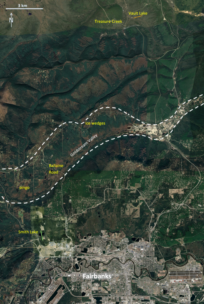
Scientists and citizens took great interest in the Goldstream Valley AEM dataset’s ability to map permafrost in 2D and 3D just north of Fairbanks, Alaska (Emond, 2018a). Figure 1 shows the general location of the example presented in this article.

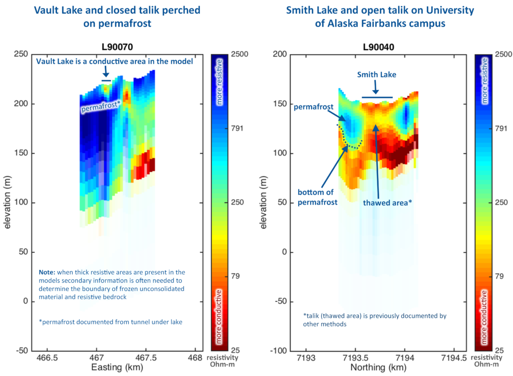
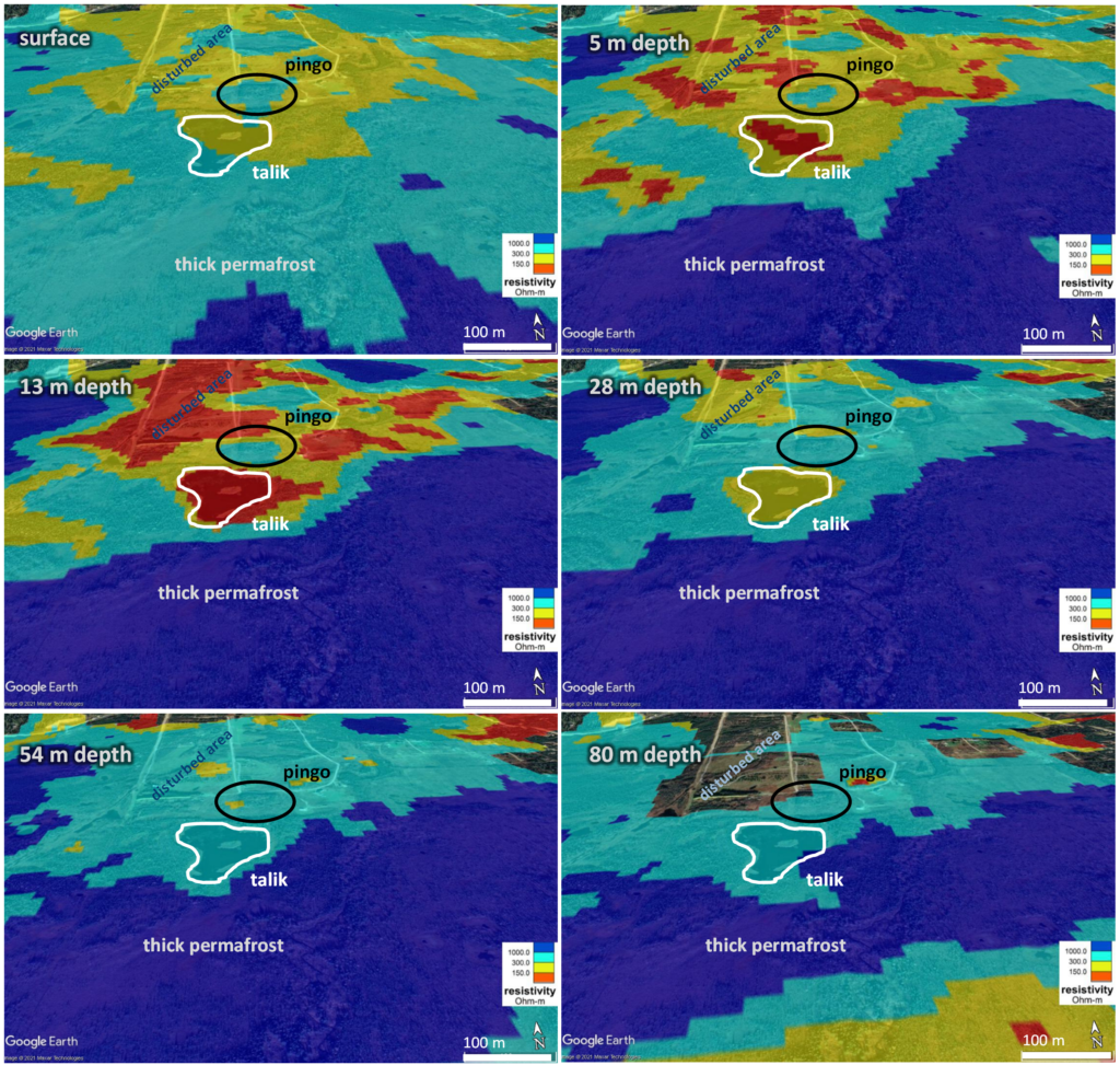
Figure 1. Permafrost — **Figure 1.** Location map of data examples near Fairbanks, Alaska.

Rapidly produced preliminary-data-derived inversion models allowed scientists to quickly target potential open taliks (thawed-through areas) to place monitoring equipment for hydrological and carbon-release studies (Walter et al., 2018). Isotope analysis of oxygen and hydrogen was used to determine if the water of select talik lakes in the Goldstream Valley study area contain a mix of ground water and meteoric water (open taliks) or just meteoric water (closed taliks). Figure 2 shows example preliminary data resistivity models of open and closed taliks (thawed area perched on permafrost) within the Goldstream Valley AEM survey.

Figure 2. Permafrost — **Figure 2**. Two resistivity model cross sections created using preliminary data of the Goldstream AEM survey.

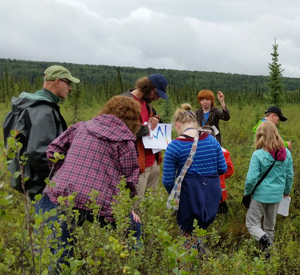
Preliminary resistivity models were shown at two public meetings, allowing citizens to look at results in their area of interest (often their property). To accomplish this, DGGS staff brought laptops with flight path .kml layers for viewing in Google Earth and 2D resistivity models cross sections of each flight line. These data are available as part of the Goldstream Valley survey publications (Emond, 2018a). Once an area of interest was identified, the appropriate resistivity model cross section was viewed and discussed. DGGS also led an educational field trip for local middle school students in Goldstream Valley, touring permafrost sites and showing 2D resistivity models for each site (Figure 3). It didn’t take long for interpretations to be made!

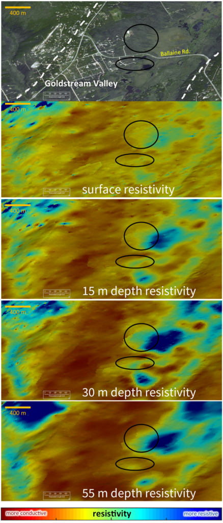
Figure 3. Permafrost — **Figure 3.** Ronald Daanen showcasing a 2D resistivity model to middle school students and two industry geophysicists. Students are standing on tall grass tussocks, a vegetation indicative of cold permafrost with a thin active surface layer. The resistivity model in this location shows a thick resistor.

Surface talik thickness can be interpreted from the Goldstream Valley survey resistivity models. Figure 4 shows variable surface talik thickness in the Ballaine Road area of the survey. The surface talik layer is a permanently thawed area above permafrost and below the active layer that does seasonally freezes to a depth of one to two meters in the Goldstream Valley. Areas of thinner and thicker permafrost are also identifiable in the models presented in Figure 4. A pingo in the central Goldstream Valley makes a clear signature in the first 15 meters of the resistivity models. Decreased resistivity is observed in relation to the talik and residential areas shown in Figure 5.

Figure 4. Permafrost — **Figure 4.** Aerial image and resistivity model depth slices of the Ballaine Road area, Goldstream Valley. Two permafrost transition zones are marked with ellipses. Thin active layers are present on right side of ellipses closer to the center of the valley. Thick active layers and thinner permafrost are present as elevation gradually increases towards the edge the valley on the left side of the ellipses. The bottom of permafrost can be seen as a reduction in resistivity in the 55 meters below ground surface depth slice.

Figure 5. Permafrost — **Figure 5.** Pingo, perched talik, and disturbed areas example. Six resistivity model depth slices are draped over topography and displayed in an oblique view. A pingo, a perched talik that rest on top of permafrost, and an area of thick permafrost are labeled. The circled pingo is a 15-meter-high hill in the otherwise flat valley. The pingo shows as an area of high resistivity in the surface, 5 m, and 13 m resistivity models. In contrast the thawed water of the lake and talik have low resistivity values. The thick, cold, and undisturbed permafrost of the central valley has the highest resistivity. Low resistivity values can be seen in the upper portions of the shallower depth slices surrounding residential development.

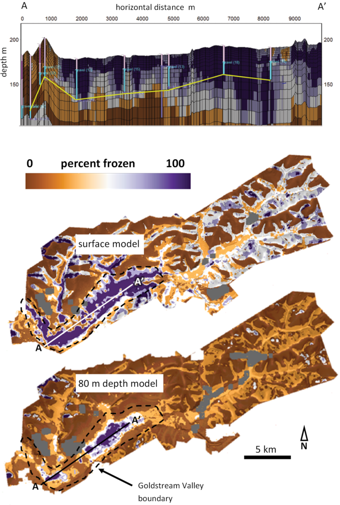
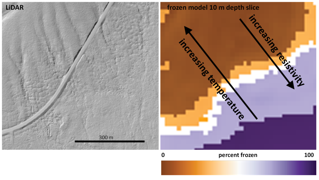
The 3D resistivity model, drilling results, isotope analysis, vegetation, and surficial morphology were used to create a frozen-thawed model for the Goldstream Valley (in progress). The cross section and map views show thinner permafrost in the western portion (Figure 6). The frozen-thawed model correlates well to an area of ice wedge degradation shown in Figure 7. Ice wedges form from seasonal contraction cracks of frozen soils that are then filled with meltwater. Over time these wedges can create polygonal areas of lower ice content material bounded by linear ice wedges. When local temperature warms the ice, wedges lose more volume leaving polygons of elevated ground. These areas of ice wedge degradation can be detected and visualized with LiDAR data.

**Figure 6.** Cross section (top) and two map views (bottom) of frozen state of unconsolidated material across Goldstream Valley. The frozen state was modeled using resistivity values and a lithologic model generated from boreholes and elevation. On the cross section are 10 historic wells with borehole logs. The yellow line represents the permafrost depth from these wells. In some cases, these wells did not reach the bottom of permafrost. The borehole data is from the 1930s and 1940s from gold exploration. On the left part of the cross section and map views or the lower part of the watershed the permafrost is thinner and of lesser extent. We believe that fire caused a disturbance in the permafrost distribution and temperatures.

**Figure 7.** Ice wedge degradation. LiDAR data (DGGS Staff, 2013) and frozen model 10 m depth slice. The transition from frozen to thawed correlates well to areas of ice wedge degradation seen in the LiDAR data as linear depressions surrounding polygons of higher ground (DGGS Staff, 2013) .

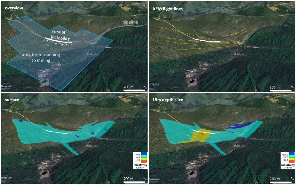
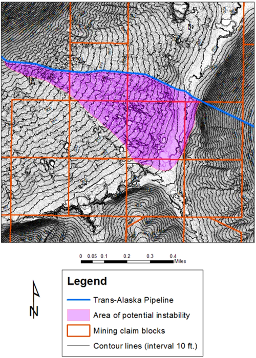
The Goldstream Valley AEM survey data also covers an area of the Trans-Alaska Pipeline System (TAPS) that has measured, monitored, and manageable ground movement. The State of Alaska wanted to reopen the Treasure Creek area downslope of the pipeline to mining and consulted DGGS for guidance on where land potentially could be reopened. Alyeska Pipeline Service Company provided sparse borehole-temperature data near the TAPS. Areas of elevated conductivity correlated well with higher borehole temperatures and ground movement. Using this correlation, the resistivity models effectively mapped the extent of degrading permafrost (Figure 8) and determined the degrading permafrost as the cause of ground movement. Stable permafrost free ground is found upslope (north) of the area of instability. The higher elevation south facing ground is warmer and has less loess accumulation. DGGS recommended no surface or subsurface disturbance should take place near the area of instability (Figure 9 as disturbances accelerate permafrost degradation.

**Figure 8.** Treasure Creek study area. Project area and area evaluated for mineral entry re-opening (polygon), Trans Alaskan Pipeline (gray line), and area of GPS measured instability (orange line with arrows). Airborne electromagnetic data flight lines (Emond and others, 2018a). The resistivity model depth-slice grids were produced from stitched 1D inversions produced by Aarhus Workbench. The area of reduced resistivity in the 19-meter depth slice correlates with elevated borehole temperatures and downslope ground movement. The surface resistivity is high as the survey was conducted during early March when the first one meter was frozen.

**Figure 9.** Treasure Creek instability map. Potential instability area was determined using AEM and subsurface data. Topographic contours from LiDAR elevation model (Hubbard et al 2011). DGGS recommended closure of claim blocks adjacent to the area of potential instability.

CONCLUSIONS

Examples from DGGS’ AEM surveys show the utility of AEM data to differentiate cold (healthy) permafrost from thawed and degrading areas, identify potential open taliks, map permafrost thickness and extent, and identity pingos.

ACKNOWLEDGMENTS

Funding for these data were provided by the National Science Foundation, U.S. Geological Survey, State of Alaska, and U.S. Bureau of Land Management.

REFERENCES

Burns, L.E., Graham, G.E., Emond, A.M., Stevens Exploration Management Corp., and Fugro Airborne Surveys, 2020, Alaska Highway corridor electromagnetic and magnetic airborne geophysical survey data compilation: Alaska Division of Geological & Geophysical Surveys Geophysical Report 2020-15, 17 p. https://doi.org/10.14509/30462

DGGS Staff, 2013, Elevation Datasets of Alaska: Alaska Division of Geological & Geophysical Surveys Digital Data Series 4, https://maps.dggs.alaska.gov/elevationdata/. https://doi.org/10.14509/25239

Emond, A.M., Daanen, R.P., Graham, G.R.C., Walter Anthony, Katey, Liljedahl, A.K., Minsley, B.J., Barnes, D.L., Romanovsky, V.E., and CGG Canada Services Ltd., 2018, Airborne electromagnetic and magnetic survey, Goldstream Creek watershed, interior Alaska: Alaska Division of Geological & Geophysical Surveys Geophysical Report 2016-5, 14 p. http://doi.org/10.14509/29681

Auken, E., Christiansen, A. V., Kirkegaard, C., Fiandaca, G., Schamper, C., Behroozmand, A. A., et al, 2015, An overview of a highly versatile forward and stable inverse algorithm for airborne, ground-based and borehole electromagnetic and electric data. Exploration Geophysics, 46(3), 223–235. https://doi.org/10.1071/EG13097

Emond, A.M., Daanen, R.P., Graham, G.R.C., Walter Anthony, Katey, Liljedahl, A.K., Minsley, B.J., Barnes, D.L., Romanovsky, V.E., and CGG Canada Services Ltd., 2018a, Airborne electromagnetic and magnetic survey, Goldstream Creek watershed, interior Alaska: Alaska Division of Geological & Geophysical Surveys Geophysical Report 2016-5, 14 p. https://doi.org/10.14509/29681

Emond, A.M., Little, L.M., Graham, G.R.C., Minsley, B.J., and CGG, 2018b, Airborne electromagnetic and magnetic survey, Yukon Crossing, interior Alaska: Alaska Division of Geological & Geophysical Surveys Geophysical Report 2016-4, 3 p. https://doi.org/10.14509/29682

Emond, A.M., Minsley, B.J., Daanen, R.P., Graham, G.R.C., and CGG, 2018c, Airborne electromagnetic and magnetic survey, western Yukon Flats, interior Alaska: Alaska Division of Geological & Geophysical Surveys Geophysical Report 2016-2, 3 p. https://doi.org/10.14509/29683

Graham, G.R.C., Emond, A.M., Daanen, R.P., Minsley, B.J., and CGG, 2018, Airborne electromagnetic and magnetic survey, Yukon Crossing to Fox profile, interior Alaska: Alaska Division of Geological & Geophysical Surveys Geophysical Report 2016-3, 3 p. https://doi.org/10.14509/29684

Hubbard, T.D., Koehler, R.D., and Combellick, R.A., 2011, High-resolution lidar data for Alaska infrastructure corridors: Raw Data File RDF 2011-3, Alaska Division of Geological & Geophysical Surveys, Fairbanks, Alaska, United States.

Mikucki, J. A., Auken, E., Tulaczyk, S., Virginia, R. A., Schamper, C., Sorensen, K. I., et al., 2015. Deep groundwater and potential subsurface habitats beneath an Antarctic dry valley. Nat Commun, 6. Retrieved from http://dx.doi.org/10.1038/ncomms7831

Minsley, B. J., Abraham, J. D., Smith, B. D., Cannia, J. C., Voss, C. I., Jorgenson, M. T., et al., 2012. Airborne electromagnetic imaging of discontinuous permafrost. Geophysical Research Letters, 39, L02503. https://doi.org/10.1029/2011GL050079

Minsley, B.J., Emond, A.M., and Rey, D.M., 2017, Airborne electromagnetic and magnetic survey data and inverted resistivity models, western Yukon Flats, Alaska, February 2016: U.S. Geological Survey data release, https://doi.org/10.5066/F7QC01P9

Olhoeft G.R., 1978. Electrical properties of permafrost: Proc. 3rd International Conference On

Permafrost. Natural Resources Council, Canada.

Rey, D. M., Walvoord, M., Minsley, B., Rover, J., & Singha, K., 2019. Investigating lake-area dynamics across a permafrost-thaw spectrum using airborne electromagnetic surveys and remote sensing time-series data in Yukon Flats, Alaska. Environmental Research Letters, 14(2), 025001. https://doi.org/10.1088/1748-9326/aaf06f

Vanhala, H., Petri, L., Antti, O., 2009, Electrical Resistivity Study of Permafrost on Ridnitšohkka Fell in Northwest Lapland, Finland, Geophysica (2009), v. 45(1–2), p. 103–118, Geological Survey of Finland, Betonimiehenkuja4, FIN-02150 Espoo, Finland

Walter, A.K., Schneider von Deimling, T., Nitze, I., Frolking, S., Emond, A., Daanen, R., Anthony, PP., Lindgren, P., Jones, B., and Gross, G., 2018, 21st-century modeled permafrost carbon emissions accelerated by abrupt thaw beneath lakes, Nature Communications, v. 9, p. 32–62. https://doi.org/10.1038/s41467-018-05738-9

BIOS

Abraham Emond ([email protected])

Office 907 451 3098

Mobile 801 839 4127

Abraham is a staff geophysicist Alaska Division of Geological & Geophysical Surveys. He is responsible for the distribution, promotion, publication, and archiving of the DGGS geophysical data collection. These data are critical to Alaska’s resource exploration, transportation, and environmental stakeholders. Abraham also manages the acquisition of new geophysical data for the benefit of the State of Alaska. His specialty is potential field geophysics including magnetic, electromagnetic, gravity, and radiometric methods. He assists the division with data type selection, survey design, data interpretation, and data modelling for a variety of applications with a focus on mapping, resource exploration, and permafrost. Prior to joining DGGS Abraham worked as a mineral exploration geophysicist. Abraham earned his M.Sc. from the University of Utah and his B.Sc. from the Colorado School of Mines. Prior to graduate school Abraham worked in the UXO industry.

Ronald Daanen ([email protected])

Office (907) 451 5965

Mobile (907) 371 6253

Ronald is a cold climate hydrologist focusing on permafrost, vadose zone physical/chemical/biological processes, slope stability, programming and modeling, wastewater treatment, drainage systems, groundwater resources, and water flow in snow. Ronald’s main task for the division is quantifying groundwater resources in Alaska. Climate change is changing permafrost through out the state which is a major restriction top groundwater flow and makes quantifying groundwater recharge challenging. Climate change is making groundwater resources more valuable in the United States as arid regions are becoming more arid and water needs are growing. Prior to working for DGGS Ronald received his B.Sc in environmental engineering in Groningen, NL; a M.Sc. in Agricultural Hydrology from Wageningen University, NL; a Ph.D. from the University of Minnesota in water resources. Ronald also worked for a decade at the University of Alaska Fairbanks studying Permafrost.

Burke Minsley ([email protected])

Office (303) 236 5718

Burke Minsley joined the USGS in 2008 as a Research Geophysicist with the Geology, Geophysics, and Geochemistry Science Center in Denver, Colorado. After receiving a B.S. in Applied Physics from Purdue University in 1997, Burke began his career as a field geophysicist working on offshore seismic vessels before receiving a Ph.D. in Geophysics from MIT in 2007. His work involves the development and implementation of innovative ground-based and airborne geophysical methods used in interdisciplinary studies to improve our understanding of Earth’s geosphere, hydrosphere, and cryosphere. Burke’s projects are interdisciplinary and geographically diverse, including permafrost mapping in Alaska, critical zone studies in a mountain headwater system in Colorado, and a large regional water availability study in the lower Mississippi River valley. He also works on development of computational methods for uncertainty quantification in geophysical datasets and associated geologic or hydrologic interpretations. In 2012, Burke received the PECASE award for his fundamental research on advancing airborne electromagnetic survey methodology and its use in studying permafrost. He is currently serving as President of the Near-Surface Geophysics Section of AGU from 2021-2022.