
By Kate McKinley1 and Alex Balog1
1 THG Geophysics, Murrysville, Pennsylvania
Introduction
With the recent increase in utility-scale solar projects, engineers are faced with the challenge of determining the appropriate foundation design in geographic areas dominated by variable shallow subsurface conditions. Typically, information to aid in foundation design is obtained through geotechnical drilling programs. However, the scale of the project and variation in the shallow subsurface minimizes the value of point data generated from high cost drilling programs. These drilling programs generate highly detailed vertical subsurface records but have low spatial resolution resulting in a model that may omit localized shallow variations. This is especially true when constructing solar projects over highly weathered carbonate bedrock where dissolution and other karst-related processes result in bedrock topography that varies greatly over short lateral distances.
Geophysical investigations have always served to supplement drilling programs, but the shallow, large-scale problem facing engineers in solar project design has introduced new challenges that geophysical techniques are uniquely apt to solve. The typical excavation zone of a solar project is within 20 feet of the ground surface. If bedrock is expected to vary between 5-20 feet below grade, contactless techniques like terrain conductivity mapping (TCM) are ideal for rapidly mapping subsurface conductivities that can be used to differentiate specific subsurface conditions. If bedrock is expected to vary between 0 to 8 feet below grade, the vertical resolution of TCM may not match the design needs of the foundation engineers. Sites exhibiting very shallow variations will need to be assessed using ground penetrating radar (GPR). GPR is a powerful imaging tool that can rapidly acquire data, but is limited by soil conditions and data processing time. The introduction of 3-D GPR arrays with its increased data collection makes GPR more feasible for large scale projects. 3-D GPR array data acquisition and increased sampling frequency amplifies the signature of deep data, and advanced data processing makes volumes of data faster to analyze than individual profiles.
Geophysical Instruments
GF Instruments multi-dipole terrain conductivity meters are ideal tools to image the shallow subsurface. The CMD Explorer is a 15-foot long cylinder containing a transmitter and three sets of receiving coils at dipole separations of 4.9, 9.3, and 14.7 feet and the Explorer 6L has 6 sets of receiving coils at dipole separations of 1.9, 3.4, 5.2, 8.0, 10.8, and 13.8 feet allowing for a penetration depth of up to 30 feet. When paired with digital global positioning system and mounted on an all-terrain vehicle, data can be acquired at speeds of up to 12 miles per hour, allowing for rapid high-resolution data collection.
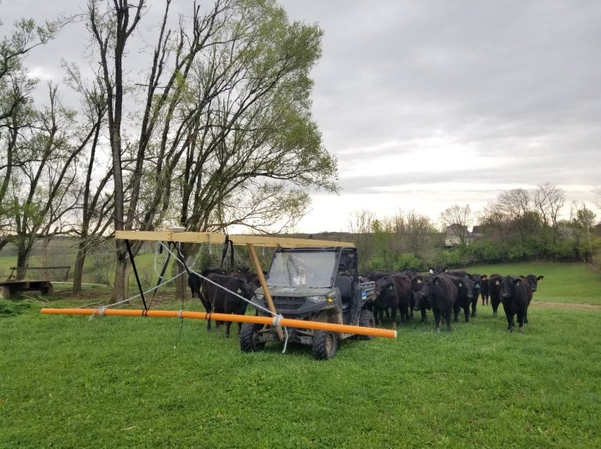
Figure 1. The GF Instruments CMD Explorer mounted on a UTV.
Impulse Radar Raptor® 18 channel array is used to acquire 3-D GPR data. The array consists of 8 transmitters and 9 receivers configured in a staggered offset array with approximately 1.5-inch line spacing between them. These antennas have a center frequency of 450 MHz and employ real-time sampling technology providing a faster data collection rate that lowers the system noise floor and effectively increases the signal penetration depth. When paired with a differential global positioning system and mounted on an all-terrain vehicle, data can be acquired at speeds of up to 10 miles per hour in farm fields.
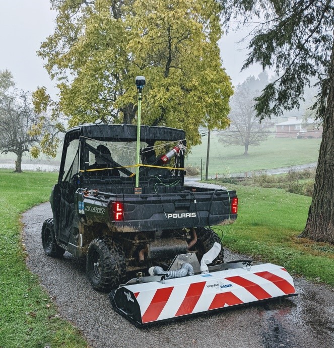
Figure 2. The Impulse Radar Raptor® 3-D 18-channel GPR array.
Case study: Terrain Conductivity Mapping
A TCM survey of a 35-acre portion of a larger solar project, consisting of rolling agricultural fields, was acquired during the off-season to avoid crop damage and potentially difficult conditions for survey collection.
At this site, the subsurface consists of clay and sandy soils underlain by fine- to coarse-grained, horizontal, thin- to medium-bedded limestones. Some thin-bedded shales also occur throughout the formation.
The CMD Explorer collected approximately 15,200 measurements with a line spacing of 40-60 feet and 1.5 feet between data points along the lines in approximately 2 hours. TCM quadrature phase measurements were converted to resistivity for post-processing and inversion using Aarhus Workbench software (AGS 2021a) in about 8 hours.
Processing resistivity data consists of several steps designed to improve the signal-to-noise ratio, allowing for a more successful inversion. Negative data and noisy data due to coupling with metal fences and buried utilities were removed. The data was averaged using a median filter with a length of 3 meters. Client-provided LiDAR elevation data were applied to each measurement for accurate vertical positioning.
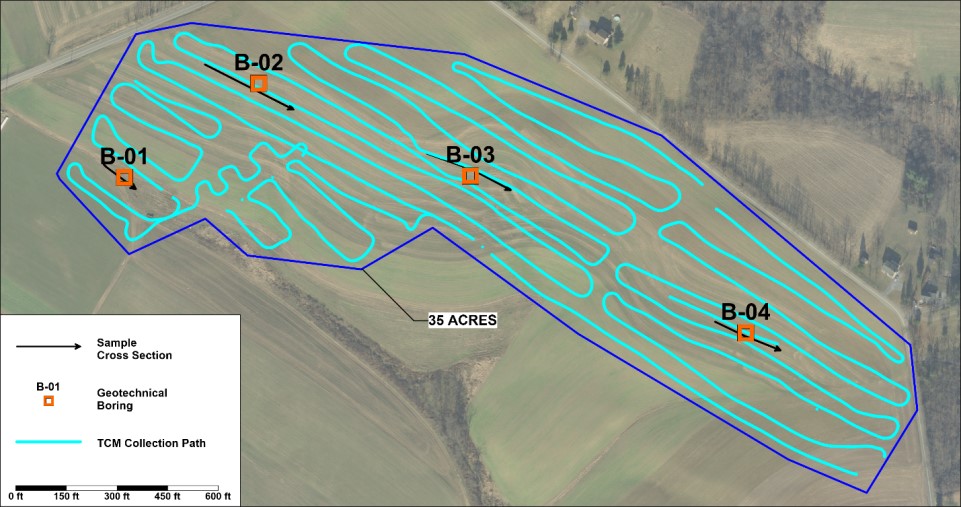
Figure 3. Map of UTV-mounted TCM collection paths. Cyan lines represent collection paths with the GF Instruments CMD Explorer terrain conductivity meter. Orange squares represent the location of geotechnical borings. Black lines represent cross sections generated from processed and inverted data and used to compare resistivity data against known boring data.
Processed data were inverted with a smooth 15-layer model, spatially constrained inversion (SCI) algorithm. An SCI is a 1-D inversion with 3-D constraints. There are constraints on resistivity along survey lines, between survey lines, and between vertical model layers. The strength of spatial constraints is scaled linearly with distance, effectively disabling constraints between measurements that are far from one another.
Post-processing and inversion resulted in approximately 15,000 locations that contain variable-depth resistivity values. To extract useful information such as depth to bedrock from this data, associations must be made between known boring data and resistivity.
To accomplish this, cross sections are drawn over existing borings and relevant boring data are overlaid on the profiles. The resistivity values at the transition from soil to bedrock are recorded. For this site, this transition occurs at 50-80 Ohm-m. Once the resistivity values at the transition from soil to bedrock are known, a weighted cutoff filter can be applied to the entire dataset using this range as the search criteria (AGS 2021b). This cutoff filter queries each individual vertical resistivity model and extracts the depth and elevation where the criteria are met. These data are then interpolated to generate modeled depth to bedrock maps. For this site, the depth to bedrock maps exhibit a highly variable subsurface caused by the presence of uneven weathering of carbonate bedrock.
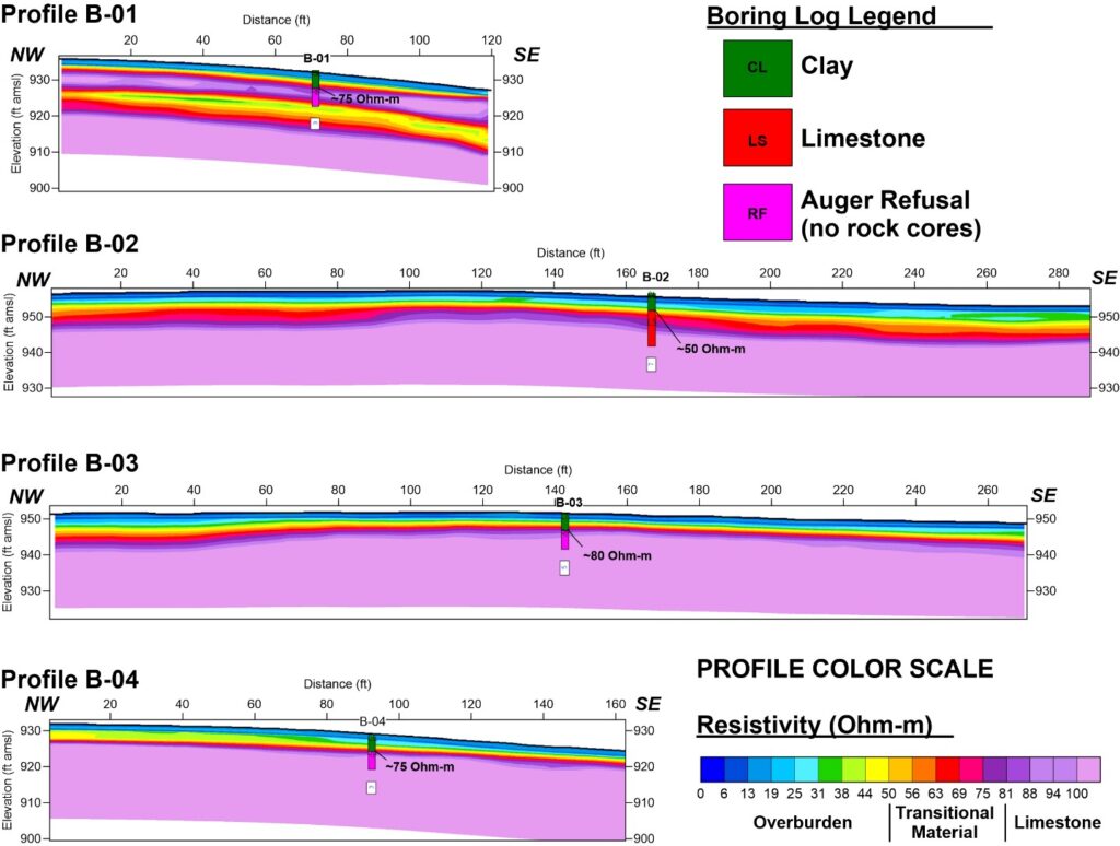
Figure 4. Cross section of inverted resistivity data derived from TCM measurements. Existing boring data are overlain onto the profiles.
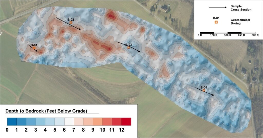
Figure 5. Depth to bedrock map derived from TCM data. GIS integration allows for depth to be displayed in either units of feet below grade or elevation above mean sea level.
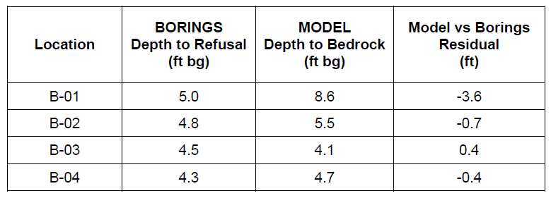
To evaluate the relative success of the model, known bedrock depths from boring data are compared against modeled bedrock depths. The resulting residual difference is interpolated to generate a contour map highlighting the relative success of the model. For this site, approximately 85% of the area surveyed was mapped to within ±1 foot of known bedrock depths.
Although the results of TCM surveys offer an impressive leap in horizontal spatial resolution compared with traditional 2-D geophysical methods and drilling programs, solar project designers are often seeking depth to bedrock maps within ±6 inches of data residual. GPR is an ideal tool for high resolution mapping, but single channel data collection and processing time is substantial.
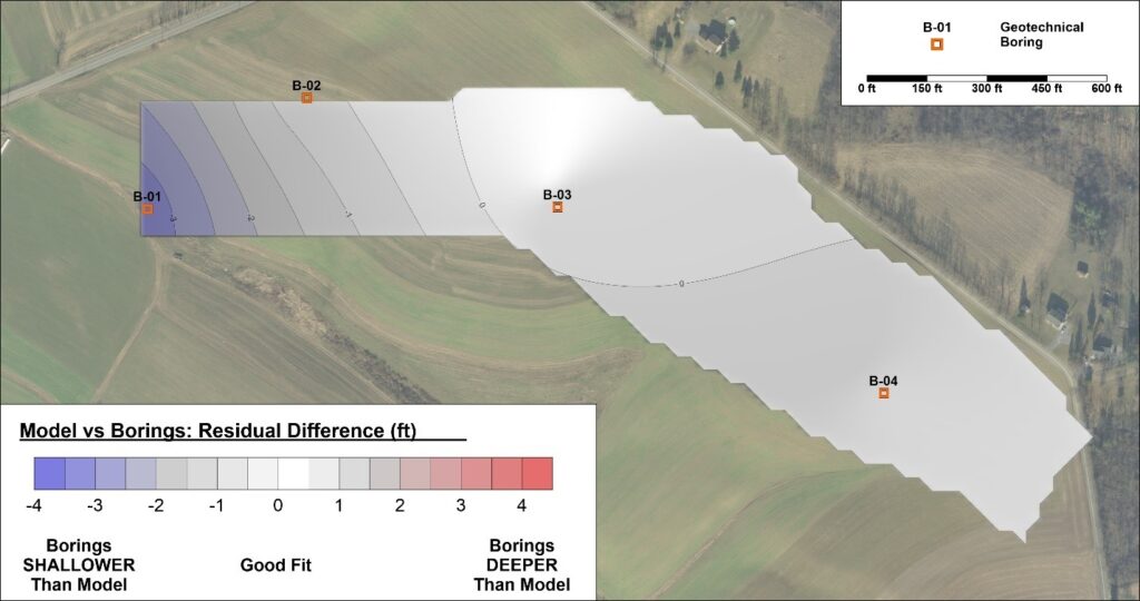
Figure 6. Residual difference between modeled depth to bedrock and known depth to bedrock from geotechnical boring data.
Case study: 3-D GPR
Impulse Radar Raptor® (ImpulseRadar, 2018) was employed to map the presence of shallow bedrock in a 1-acre section of a project where TCM indicated bedrock was near the ground surface. The project site consisted of a sloped, grass-covered agricultural field accessed during the off-season to avoid crop damage. The subsurface consists of clay soils underlain by thin-bedded shales. Additionally, a sloping utility traverses the field in the study area.
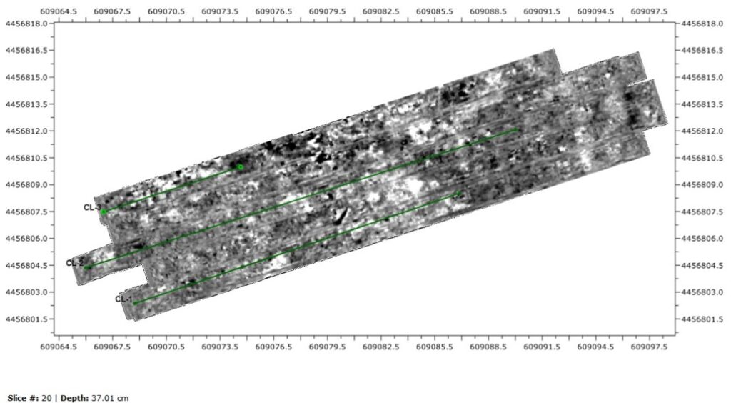
Figure 7. Map of UTV-mounted Raptor collection paths. GPR array data at 15 inches below ground. Green lines represent the location of GPR data cross sections.
Data collection was completed in swaths with one channel of overlap to ensure complete coverage in one half hour. Data positioning was controlled using a differential GPS setup with a local base station and a rover attached to the array.
The Talon acquisition software provides the configuration and control of the antennas for quality control of the GPR data and the positioning data during acquisition. Color-coded status indicators allow for easy observation of the hardware components including the condition of each measurement channel and incoming positioning data, so that signal performance and proper operation can be monitored. Views can be toggled between the radar data acquisition screen and the navigation map view. To ensure optimum data acquisition, the navigation view is used to align measurement swaths correctly and to minimize gaps in the data.
Processing, visualization and interpretation of the Raptor array data was completed through Impulse Radar’s proprietary Condor software package (ImpulseRadar, 2021). Upon import, data positioning can be reviewed to detect troublesome areas with low data density, to delete incorrect positioning points, and to define parameters for positioning data interpolation. At this stage, 3-D GPR data provides additional benefits over traditional 2-D GPR profiles as it generates a volume of continuous GPR data. This allows for cross-sections to be drawn in any orientation over the area surveyed, regardless of the orientation of collection swaths. Additionally, data may be viewed in plan view depth slices or 3-D ribbon box displays of specific areas of interest. These options provide valuable insight for evaluating the quality of signal processing steps to get the most information out of the data.
These data were filtered to remove noise and improve data quality and regularized to interpolate traces across swaths. The data migration process was maximized with a migration test function that allows for simple velocity adjustment and observation of the direct effect on hyperbolas. A final post processing flow is offered to improve the image.
Interpretation of GPR data can be made directly in the software by picking lines, points or plates that can be exported directly to AutoCAD. Additionally, image and video exports are easily generated for easy end-product review.
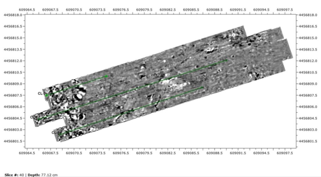
Figure 8. GPR array data at 30 inches below ground. Data maps shallow bedrock and numerous point targets. Green lines represent the location of GPR data cross sections.
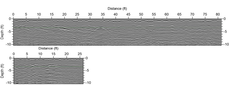
Figure 9. GPR cross sections mapping shallow bedrock and numerous point targets.
Conclusion
Depending on the expected depth to bedrock and required accuracy, TCM and 3-D GPR surveys are complementary and efficient methods for mapping depth to bedrock at large-scale solar projects. Using multi-dipole terrain conductivity meters to map variations in the shallow subsurface is fast, efficient, and results in highly detailed maps and profiles. When combined with existing geotechnical boring data, the depth to bedrock may be accurately estimated. This high-resolution information can be used by engineers when designing solar panel foundations and calculating cut-and-fill requirements. Providing residual differential maps that compare model depths to known depths from boring data indicate the degree to which models can be trusted. When TCM cannot provide enough vertical resolution in the very shallow subsurface, GPR array data is an efficient means of providing more detailed information. Supplementing existing geotechnical design programs with these geophysical techniques provides a fast and cost-effective means of increasing the amount of information available to engineers when designing a project.
References
AGS Aarhus GeoSoftware. (2021a). Inversion of ground conductivity meter data for mapping of raw materials, Skolegade 21, 1, 8000 Aarhus C, Denmark.
AGS Aarhus GeoSoftware. (2021b). Workflow for import, processing, inversion and presentation of frequency domain GCM/HEM data in Aarhus Workbench, Skolegade 21, 1, 8000 Aarhus C, Denmark.
ImpulseRadar. (2018). Raptor®-45 User Manual v.1.4, Malå, Sweden.
ImpulseRadar. (2021). Condor User Manual v.1.5, Malå, Sweden.
Author Bios

Kate McKinley is a Senior Geophysicist and Vice President at THG Geophysics, a full service geophysical firm dedicated to mapping the shallow subsurface and to providing utility location services. With nearly 20 years of experience in geophysics and business development, Kate still enjoys the everyday adventure of applying the principles of physics to imaging what lies below the surface. She has, gratefully, had the opportunity to provide these services to diverse projects in engineering, environmental, and archaeological disciplines.
Kate enjoys sharing her experiences through teaching, helping to develop her trade through her activity in several professional organizations and helping her community by participating in several local, civic organizations. ksm@thggeophyscis.com
Alex Balog is a Lead Geophysicist at THG Geophysics, Ltd. He serves as a technical resource designing and deploying conventional field surveys, processing and interpreting geophysical data. He also manages project reporting.
Alex supervises several landfill and industrial site monitoring contracts and serves as THG’s technical developer implementing new software and equipment with the company. Alex holds a Bachelor of Science degree in Environmental Science from Franklin and Marshall College in Lancaster, Pennsylvania.