
Geoff Pettifer,
editorfasttimesnewsmagazine@gmail.com
TSF Leakage Temporal Changes – A Case Study
Introduction
This edition of the Hydrogeophysics and Environmental Geophysics column focuses on the dynamic nature of TSF leakage plumes on mine sites. This is illustrated by a case study graciously provided by a mining company who for confidentiality reasons wish the mine, the location and company to remain anonymous. The case example has been submitted by the mining company in the spirit of helping to educate the industry about the dynamic nature of TSF leakage as illustrated by mapped variations in apparent EC from four EM31 surveys around the TSF, carried out over a 12 year period of the mine history.
The Nature of Tailings Dam Leakage
All tailings dams leak and the mine management operation seek to manage and monitor this leakage, according to the mining license conditions, the local environmental regulations and the mine environmental plan. Leakage plume monitoring is achieved by a combination of use of mine monitoring bore networks and electrical geophysical surveys. Single or multi-frequency or time-domain electromagnetic (EM) ground surveys are quicker, more economical and more widely used than DC electrical survey methods. Although lately airborne EM is also increasing being used, to define the extent and geometry of a TSF leakage plume. The plume management is achieved by a combination of strategically placed drainage works and dewatering bores with the intercepted plume waters often recycled back into the ore processing stream.The dynamics of TSF leakage and leakage plume characteristics is dependent on:
• mine ore processing throughput,
• changes in processing water electrical conductivity (EC) affecting plume water EC,
• which part of the TSF is utilized for tailings disposal at which time,
• deterioration over time of the containment capacity of the designed impermeable barriers in the TSF, • implementation of TSF raises
• whether the mine undergoes extended shutdown / care and maintenance periods or not, and • installation, operation and effectiveness of interception drains and dewatering bores.
EM surveys (single or repeat surveys with monitoring bore data control are an effective tool to help manage the impact of the TSF on the environment around a TSF. EM surveys are conducted for a variety of reasons including:
• monitoring the TSF leakage status, during operation and after extended mine care and maintenance periods and/or change of mine ownership, • helping to plan extension of and optimal placement (in preferential groundwater flow paths), of the monitoring bore network and to supplement and extend the bore point data monitoring of leakage plumes, • designing and monitoring the effectiveness of leakage interceptor drainage and leakage plume bore dewatering systems, • defining leakage pre-TSF raises for the purposes of environmental regulatory approval of the TSF raise, • comparing pre-and post TSF raise leakage and therefore the leakage plume changes resulting from the progressively increasing static head of the tailing pond waters, after the TSF raise.
An EM survey taken around a TSF, represents a snapshot in time of the leakage plume and native groundwater conditions and where possible should be interpreted in relation to the history of the TSF operation and the stage of drainage management in place at the time.
Given their affordability, repeat EM surveys are a highly recommended tool for temporal TSF leakage management. In terms of social license to operate, repeat EM surveys can be used by mine management to demonstrate to the regulators, the due diligence undertaken with environmental management of the mine, in particular of the TSF.
The Geonics EM instruments: the EM31 and to a lesser extent the EM34, have historically been widely used for shallow contaminant plume mapping on mining and industrial sites. The case example provided below shows how effective even a single frequency EM survey using an EM31 can be, when purposely used in repeat survey mode, with monitoring bore data control, to monitor the progressive history of TSF leakage and how effective efforts to contain the leakage have been.
Case Example – Four EM31 surveys around a TSF over a 12-year period
Figures 1 to 4 show four EM31 apparent conductivity (0-600 mS/m) maps (arbitrary local grid metric coordinates), around the northern, eastern and southern edges of an operating mine TSF over a 12-year, monitoring period. EM31 surveys with
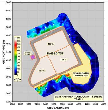
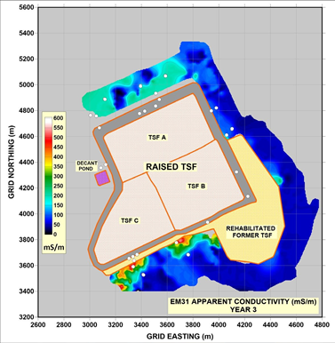
two calibrated EM31 instruments were undertaken in Year 1 (baseline survey) and Year 3 by a previous owner and in Years 9 and 12, by a new previous owner. Local geology is variable thickness recent sandy sediments / soils overlying weathered bedrock of mafic rocks (western third of the TSF) granite (the eastern two-thirds of the TSF).The purpose of Figures 1 to 4 is just to show the dynamic nature of the TSF leakage plume, without discussing the history of the
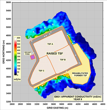
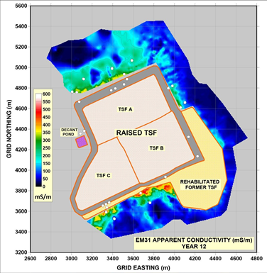
TSF operation in detail, which is beyond the intended scope of this case example presentation. Suffice to say the history of the TSF and therefore, the reasons for changes in EM31 anomalies during the 12-year period, is complex. The 12-year period was marked by change of mine ownership, change in ore processing throughput, long and short periods of mine shutdown, changes in the source salinity of the high salinity processing water, as well as progressive implementation of
various interceptor drainage works and new dewatering bores and temporal changes in utilization of cells TSF A, TSF B and TSF C of the raised TSF. Partially underlying the raised TSF is a rehabilitated former TSF which was not surveyed with the EM31 because of the disturbed and saline nature of that area of the site. Only the impact on surrounding natural ground surface and native vegetation was of concern in terms of environmental management objectives. Some of the plume management / interception interventions were guided by and were reasons for commissioning the repeat EM31 surveys and monitoring the impact of the interventions.
Groundwater Conditions affecting the EM31 results
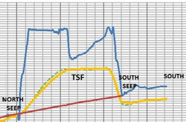
A north to south cross-section through the turkey’s nest TSF structure shows the groundwater mound from tailings water leakage (Figure 5 – explanations in the caption).
Blue- Turkeys nest TSF topography (1 metre elevation per vertical scale division). The TSF is 37 metres above natural surface on the north side and 28 metres above natural surface on the south side; Brown – estimated original land surface pre-TSF; Yellow – interpolated groundwater table mound under the TSF assuming the shallow groundwater table is perched and independent of the nearby mining pit cone of depression (deeper groundwater table). Green dashed – interpolated groundwater table mound under the TSF assuming the shallow groundwater and deeper groundwater table are one and the same. The groundwater mound standing water level is up to 18 metres above regional natural shallow water table levels and is centred beneath the active southern TSF cells TSF B and TSF C, not the full and now dormant northern cell TSF A.
The dry unsaturated zone is very low conductivity (high resistivity sandy, dry and generally low clay content sediments), and the saturated water table zone is very highly conductive due to naturally highly saline groundwater and more highly saline TSF leakage plume waters).
The process water and the local groundwater system EC is highly saline (50,000 to 140,000 EC units of uS/cm). genrally well above seawater salinities.
Sensitivity of EM31 apparent conductivity to groundwater salinity and EC – Year 9 to Year 12 data.
For the purpose of this case example, the focus of the analysis of the relationship of EM31 apparent conductivity (ECa), EC of monitoring bore water and the standing water level (SWL – elevation and depth below local ground level and the root zone of at risk native vegetation) of the shallow water will be on Year 9 and Year 12 data where the groundwater data is more extensive.
The question is, given the very low conductivity unsaturated overburden and very high conductivity water table, how sensitive is the EM31 ECa reading and changes in ECa from Year 9 to Year 12 to the SWL and separately the water EC and also changes in both these groundwater parameters from Year 9 to Year 12? Can a relationship be developed and used to predict water table elevation from the ECa measurements, regardless of water table EC variations?
The previously mentioned high contrast in conductivity between the low conductivity unsaturated zone and the very high conductivity water table, is of assistance in interpreting the subtlety of changes over time in groundwater levels around the TSF. The conductivity contrast also permits deeper penetration of the EM signal of the EM31 compared to the conventional EM31 effective penetration depth wisdom of typically 4 to 7m.
An empirical analysis of the Year 9 to Year 12 EM31 ECa and groundwater monitoring bores water levels and salinities shows the relationship between:
• absolute EM31 ECa measurements and groundwater levels and salinity variation (Figure 6 to 7) and
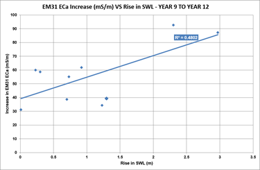
• increases in EM31 ECa versus increases in groundwater EC and increases in EM31 ECa versus changes in water levels (Figures 8 to 9)
Figure 6 shows that the relationship between EM31 ECa and bore water EC is not one simple linear relationship but is Year of
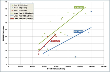
Figure 6. EM31 apparent conductivity versus Bore water EC (Red – Year 3, Blue – Year 9 and Green – Year12 data) and EM31apparent EC versus water table depth (2012 to 2015 data)
measurement dependent, reflecting the different average water table depths for a particular year of measurement (Year3, 9 or 12). The number of monitoring bores increased dramatically after Year 3 with a new ownership of the mine occurring between Year 3 and Year 9. Also the range of salinity of waters detected in the monitoring bores greatly increased after Year 3 probably reflecting more saline processing water usage.
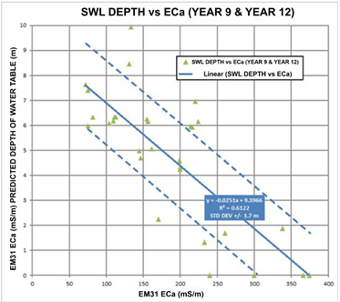
Figure 7 shows monitoring bore water table depth level data versus the EM31 ECa values. This linear relationship can be used to predict the likely depth of the water table across the area to an accuracy of approximately +/- 1.7 metres, from EM31 ECa values. This can then be used to monitor and predict high risk areas where the vegetation root zone could be impacted (depending on the root zone critical depth criteria imposed by licensing conditions).
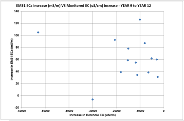
It therefore turns out that because of the strong contrast in EC between the dry unsaturated zone and the high salinities of the water table, the EM31 ECa is most sensitive to the depth of the saline water table and less sensitive to groundwater EC variations within a high EC range of values. This is also evident when relative rises in groundwater elevations occur (Figure 8 versus 9).
Figure 8 shows there is no sensible relationship between the moderate to large decrease in groundwater EC that occurred between Year 9 to Year 12 and what might be expected to be a decrease in EM31 ECa.
This type of analysis is pertinent to saline TSF waters but may not be pertinent to lower TSF water salinity situations.
Conclusions
There are two key takeaways from this case example:
1. TSF leakage is dynamic and any planned EM or resistivity monitoring of leakage variation needs to take this fact into account and to use monitoring bore data for calibration purposes to interpret what is occurring.
2. Where the processing water and the groundwater table are both very saline, useful empirical approaches can be adopted to predict water table depth from EM31 ECa.
Geoff Pettifer, editorfasttimesnewsmagazine@gmail.com