Electromagnetic Induction Sensing of Underwater Munitions: Detection and Classification with the UltraTEM system

Lin-Ping Song, Stephen D. Billings, Leonard R. Pasion, and David Sinex

Black Tusk Geophysics, Vancouver, BC, V6J 4S5, Canada

Abstract

In the complex marine environment, the detection and characterization of metallic items using electromagnetic induction (EMI) sensing face some unique physical and operational challenges. These challenges include the effects of conductive seawater, surveying altitude, navigational accuracy, coverage area, and a low signal-to-noise ratio. In this paper, we first provide a brief overview of the UltraTEM system and the processing methods we developed to address these challenges. These methods encompass modeling and characterizing conductive backgrounds, enhancing detection capabilities, and performing robust inversions even with sensor positional uncertainty. We assessed these methods using the UltraTEM marine data acquired at the designated Sequim Bay Demonstration site. We then shift our focus to the detection and classification performance of the blind test data at both low and high altitudes, highlighting insights gained from successful and unsuccessful examples in this demonstration. Our analysis and results show that marine EMI sensing has considerable potential to be deployed as a practical and effective advanced geophysical classification (AGC) tool.

Introduction

Increased human recreational and industrial activities in the offshore environment have led to more potential interactions with discarded military munitions (DMM) and Unexploded Ordnances (UXO). Over the years, a variety of sensing techniques including sonar, laser, optical, electromagnetic induction, and magnetometry have been developed to help remediate shallow water sites contaminated by munitions. Of particular is marine EMI sensing, which is adopted from the terrestrial case (Pasion and Oldenburg, 2001; Bell et al, 2001), that aims to identify and classify if detected munitions belong to UXO or clutter based on the polarizabilities (the physical property) of a target extracted from measurements. With this discriminative, diagnostic information of polarizabilities, marine EMI sensing has emerged as a promising technique for underwater munitions detection and characterization (Shubitidze, 2011; Schultz et al, 2011; Bell et al, 2016; Billings and Song, 2016).

Marine EMI sensing has some distinct physical and operational challenges. For a survey deployed in a dynamic underwater environment, strong, variable background EMI responses can be ubiquitously observed due to the conductive seawater (the conductivity around 4-6 S/m) and variations of sensor altitude and attitude. As a result, such seawater responses would inevitably obscure and distort the responses of a target of interest. With the presence of conductive seawater and limited accessibility in environmentally sensitive areas, EMI measurements taken at large standoff distances to the seafloor are likely to contain signals that are too weak to be detectable. Moreover, accurate sensor positioning of a marine EMI survey is more difficult than for the terrestrial case. Relative positional errors between adjacent survey lines can lead to an erroneous inversion and subsequent misinterpretation.

With the recent development and demonstration of underwater EMI systems, e.g., UltraTEM (Billings, et al, 2023), acquired marine EMI data are available for evaluating our developments to address technical difficulties. In the following paper, we first provide a synopsis of methods that use 1) an integral equation technique for characterizing and removing background responses; 2) a synthetic aperture scheme for enhancing target detectability; and 3) data inversion methods that are robust to sensor positioning errors. Next, the results of processing UltraTEM data collected at the Sequim Bay test-site are presented to demonstrate the effectiveness of the combination of the marine UltraTEM system and the processing methods. Finally, the conclusions follow. Below, we start with a description of the sensor system.

UltraTEM system

The UltraTEM system (for a thorough description, see Billings et al., 2023), a multi-component multi-sensor system that uses time-domain electromagnetic induction (TEM) to detect and characterize buried metal, can be deployed for both terrestrial and marine applications. The plot on the left of Figure 1 shows the sensor geometry in which the four transmitter loops and twelve tri-axial receiver cubes are mounted to the platform. For each transmitter excitation, UltraTEM records the response at all receivers. Thus, it has spatial–temporal data of 144 × N_t for a survey point, where N_t is the number of logarithmically spaced time gate measurements of transient signals. To minimize the effect of 60 Hz powerline frequency used in the United States, the system is designed to have the excitation current waveform in a transmitting loop regulated in either fast (90 Hz base-frequency) or slow (30 Hz base-frequency) modes. In the fast-transmitter mode, the transient signals may be measured ranging from 0.124ms to 2.42ms with N_t= 27; in the slow-transmitter mode, 0.124ms to 7.7ms with N_t= 37. With the three 1.8m x 1.8m transmitter loops, and one 3.6m x 0.9m overlapping transmitter loop, as well as distributed receiver cubes, the system approximately samples an effective footprint area of 4 square meters.

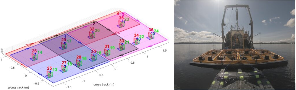
Figure 1. Left: sensor geometry of the UltraTEM: four horizontally arranged transmitters and twelve triaxial receiver cubes. Right: View of the UltraTEM and Ugly Duckling vessel from a camera mounted at the stern of the tow-fish. This photograph was taken at Lake Washington.

The sensor system is installed in a submersible tow-fish that is towed by a surface vessel. Through ESTCP MR19-5073, the UltraTEM marine towed system has been built for detection and classification of buried ordnance and designed as a vessel-towed single-pass marine dynamic classification system. The system combines RTK GNSS, ultrashort base line (USBL) acoustic positioning, and subsea inertial navigation system (INS) to provide the most precise marine positioning available. Data from the tow-fish are remotely monitored and logged via fiber optic telemetry through the tow cable using computers aboard the deployment vessel. The plot on the right of Figure 1 shows a deployment of the system at Lake Washington.

For the specific task of UXO detection and classification, the UltraTEM system has been enhanced by integrating Gap Explosive Ordnance Detection’s (GapEOD) and Black Tusk Geophysics’ (BTG) existing multi-component multi-sensor UltraTEM package and associated software into Tetra Tech’s (Tt) towed electromagnetic array (TEMA) platform. The evaluation and analysis of the system performance were reported in Billings et al, 2023. Next, we will briefly describe the methods that were developed to address the challenges aforementioned in the marine environment.

Methods

Integral equation modeling and characterizing EMI responses

In the absence of noise, the measured EMI transient responses at an instant t in seawater may be described as the sum of the conductive background fields and the scattered fields due to the presence of a buried metallic target upon excitation. The transient responses can be modelled by the integral equation (IE) method in layered media (Song et al, 2016; Billings and Song, 2020).

When surveying in a dynamic marine environment, the sensor pitch and roll as well as altitude above sea-bottom will vary. The variations of these sensor parameters change the transmitter and receiver couplings with layered interfaces and therefore influence the EMI response measured by the sensor. Our modeling and experiments show that the characteristics of EMI responses correlate well with the variations of survey parameters. The z-component of background responses is more influenced by the variation of sensor altitude, the y-component by the variation of sensor pitch, and the x-component by the sensor roll.

As an illustration, Figure 2 shows a comparison of modelled results (Tx4-Rx1Z) with data acquired at the blind-grid area of Sequim Bay. The three-layered structure is used to model the conductive background responses. The seawater depth and conductivity are set as 23m and 3.6 S/m, respectively. A homogenous half-space seabed is assumed with a conductivity of 1 S/m. The plot on the left shows the platform altitudes (Figure 2a) and depths (Figure 2b) during the survey. Figure 2c shows the observed (in Figure 2.

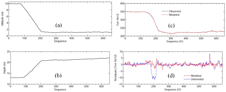
Left: Observed and modelled responses of Tx4-Rx1Z. right: Background subtracted responses with the modelling and de-trending methods.

blue) and modeled (in red) background profile at t = 0.19ms. One sees that the field amplitude decreases as the system descends deeper (Figure 2a). The conductive background responses correlate well with the sensor heights. A de-trend filter may be applied to remove the background fields. Figure 2d shows that the de-trend filter works well for smooth changes in altitude and attitude but produces a relatively large filtering artifact around the rapid changes in the observed responses. In contrast, the modeled responses well predict the observed data, including those rapid changes. Overall, the high-amplitude background can be effectively removed using the model or a de-trending filter, and an anomaly response (the spikes) can be extracted for a subsequent processing.

Enhancement of target detection: TEM synthetic aperture method

In a standard analysis, target detection is performed on a data image created by combining z-component data of all transmitters. An anomaly ‘blob’ on the data map, which has an amplitude exceeding a threshold, is identified and picked as a target. However effective target detection can become difficult due to weak strength of signals at large standoffs. To improve detection and sharpen anomalies in gridded images or along profiles, we explore a superposition approach, called synthetic aperture (SA) method (Knaak et al, 2015), that attempts to boost target signals by stacking the responses from multiple transmitters or receivers.

Assume an EMI survey that fires a transmitter at r _l (l = 1,2,⋯,L), to interrogate the subsurface. There are the receivers at r _i (i =1,2,…,N) to record the responses. Denote d_il as the response measured at the i-th receiver associated with the l-th source excitation. The idea of a SA method is to sum the responses measured by the same receiver from the excitation of all sources (ibid). The SA data at the i-th receiver associated with the synthetic source can written be as d_i,SA=∑^L_l=1w_l d_il =d _i^T w, where w=[w₁ w₂⋯w_L]^T is the vector of the synthetic aperture weights and the i-th common receiver gather given as d _i=[d_i1 d_i2⋯d_iL ]^T .

Similarly, the concept of the SA can be used to construct a SA receiver for common transmitter gathers. This shows that the reciprocity principle applies where the synthetic receiving aperture is formed by exchanging transmitting and receiving roles. In the synthetic receiving aperture, the original transmitter acts like a “receiver” and the synthetic receiver acts as a “transmitter.” The above SA process may be used sequentially to form a set of composite SA data. The SA weights are determined by maximizing the SA energy function.

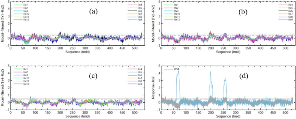
Figure 3. Example of SA detection for UltraTEM Blind-Grid data, Sequim Bay. (a)-(c) The twelve filtered vertical responses for Tx1, Tx2, Tx4. (d) SA response (plotted in cyan).

The SA method is a promising approach to boost potential target signals and thus help detection (Song and Billings, 2023). Figure 3 presents a case of applying the SA method to the UltraTEM blind-grid data collected at high altitude (about 1.5m). The regular responses of the twelve receivers’ z-coils for transmitter Tx1, Tx2, and Tx4 are shown in Figure 3a-c. Visually inspecting along the profiles, it is unclear to identify a sequence where target signals are likely present. Next, the SA method was applied to all the responses, and the generated optimal SA (OSA in cyan) responses are shown in Figure 3d. For comparison, all the responses in 3a-c are re-imposed (in gray) in Figure 3d. Along the OSA profile with a threshold of 3 mV/A, three peak anomalies were picked as the potential targets. The first pick along the profile was ignored because its location is outside of the test area. The other two were processed and analyzed. The target around sequence 200 was correctly classified as target of interest (TOI) and was confirmed to be an 81mm projectile (U224). The other target was correctly classified as a non-TOI.

Inversion by mitigating sensor positional uncertainty

Within the time range of interest, the underwater measurements can be well approximated as the superposition of the conductive background responses and target signals. Upon removing background responses from raw underwater measurements and detecting potential targets, the dipole model is readily applied for downstream processing of inversion and classification (Shubitidze, 2011; Billings and Song, 2020). Suppose that 𝜂 metallic targets are present in the sensor field of view, the measurements at time instant t are given as d(t,s)=A(α,s)β(t). Set α=(r,θ) as the locations and orientations of 𝜂 targets. The sensitivity matrix of A(α,s) relates the measurements to principal polarizations β(t). In the standard inversion method (Song et al, 2011), the locations, orientations, and principal transient polarizations, i.e., (r,θ,β(t_j)), are determined by minimizing an objective function that measures misfit between the observed data and the predicted ones. Sensing locations, correctively denoted as s, are assumed to be precisely known and not the part of the model parameters.

In a hydrodynamic environment, the actual survey track or stand-off distance from the seafloor may significantly deviate from the measured nominal one. Inaccurate relative sensor positioning between multiple survey lines can lead to an erroneous inversion of data and a poor interpretation of results. We have developed inversion methods that attempt to implicitly and explicitly account for errors in sensor positioning, respectively (Pasion and Song, 2021; Song, Sinex and Billings, 2023).

The independent model location inversion (IMLI) method assumes that the nth sensing location s_n “view” the targets as if they were at α_n=(r_n,θ_n), not necessarily at the true locations r and orientations θ. Then the standard inversion method can be modified by introducing the N sets of current extrinsic source parameters α_n, n=1,⋯,N and replacing the sensitivity matrix with A(α_n, n=1,⋯,N,s). In the joint estimation of target and survey parameters (JETSP) method, it imagines that the targets “see” through those sensing deployments and “demand” some adjustments ∆s_n of the recorded nominal position values s_n so that the adjusted sensing locations s_n=s_n+∆s_n can harmonize with the actual geometrical presence α=(r,θ) of targets. By treating the sensing location perturbations ∆s_n as additional unknowns to source parameters, the standard inversion method is modified with the sensitivity matrix A(α,s, ∆s).

We present an example of recovering two 81mm mortars (U222 and U223, PNNL-ID) from the marine blind data collected in 2022. The top panel of Figure 4 shows the observed data and three sets of the predicted data by the three methods (standard inversion, IMLI, and JETSP). The standard inversion has difficulty modelling the observed responses and yields a significant anomaly pattern in a residual map (not shown here). On the other hand, both the IMLI and JETSP fit the observed data fairly well. Perhaps the most striking difference between the standard method and the other two methods is seen on the recovered polarizabilities. As shown in the bottom panel of Figure 4, from left to right, the first set of polarizabilities recovered by the standard method may predict a target of interest with unequal minor polarizabilities. The second set of recovered polarizabilities likely predicts non-UXO, with the matching misfit of 0.864 against the 81mm reference item. On the other hand, the IMLI and the JETSP predict that the two sources have almost identical recovered polarizabilities, which match well with the 81mm reference polarizabilities. Matching misfits are 0.137 (IMLI-1), 0.222 (JETSP-1), 0.234 (IMLI-2), and 0.057 (JETSP-2).

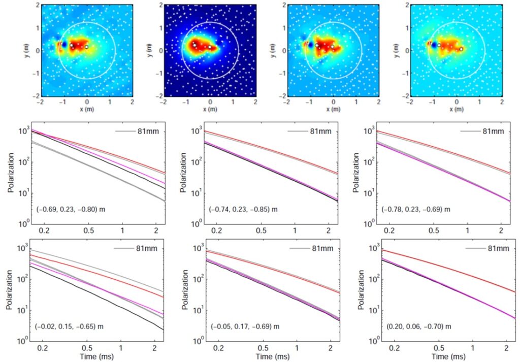
Figure 4. Example of inversions. Top: The four gridded data images show the observed and three sets of the predicted data by the standard inversion, IMLI and JETSP methods. Bottom: Recovered polarizabilities by standard inversion (left); IMLI (middle); JETSP (right). Note that the inverted source location is shown on the bottom left of each polarizability plot.

Demonstration at Sequim Bay Test Site

Site preparation and data acquisition

The UltraTEM has performed three shakedown tests. Billings et al., 2023 provided a detailed description of these tests, including experimental design, site preparation, item seeding, and the system deployment, etc. Briefly, the first two tests were conducted in Ostrich Bay and Sequim Bay, Washington in October 2021. The two tests were concerned about: 1) examining the capability of the TEMA system to deploy the UltraTEM system with acceptable stability, altitude control, and line following, and 2) evaluating performance metrics that were about location accuracy, noise and reproducibility of polarization tensor parameters. At the Sequim Bay shakedown test in 2021, UltraTEM data were collected over 0.54 Hectares, or 60% of the full Blind-Grid area. BTG processed the UltraTEM data and turned over a ranked dig-list to the ESTCP Program Office, with all 17 TOIs correctly detected and classified.

The third shakedown test was conducted in September 2022 at Sequim Bay. Two areas at Sequim Bay were undertaken by PNNL for assessing the performance of the UltraTEM system (Figure 5a). A calibration area was designed with known targets (40mm to 155mm) emplaced at known positions. The calibration data were used to examine the performance metrics, and to test the processing workflows and establish site-specific polarizability libraries. A 0.79-Hectare circular blind-test area was set up with several MEC simulants and clutter items emplaced at positions blind to the demonstration team. Calibration and blind-grid data were collected at 90 Hz and 30 Hz transmitter base-frequencies. Figures 5 (b)-(d) show the three different blind-grid surveys at lowest elevation and 90 Hz and 60 Hz transmitter mode (mode 4F and 4D) and high altitude (about 1.5m) and 90 Hz mode (4F), respectively. With 4.0m line spacing, the three blind-grid data correspond to 100%, 98.6%, and 92.9% coverage of the designed circular area.

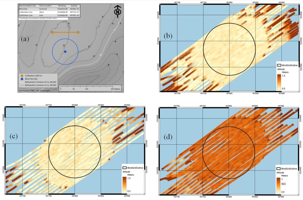
Figure 5. Data acquisition at Sequim Bay. (a) A calibration line and a blind circular test area. Survey altitudes over the blind grid area: (b) at the fast- transmitter mode and low altitude; (c) the slow-transmitter mode and low altitude; (d) the fast-transmitter mode and high altitude. Note that the color-maps have different scales. The circular black outline is the official Blind Grid area, and the solid lines are the survey tracks.

Classification

To determine if the system has the ability to detect targets of interest (TOI) to the required detection depth, we tested and applied methods to all the calibration and blind-grid data. Classification is performed by matching estimated polarizabilities to a library of polarizabilities and then ranking a target based on the matching misfit. Three ranked dig-lists were submitted to Institute for Defense Analyses (IDA) for the blind-grid tests using two datasets collected at low altitude (0.5-0.75m above the sea-bottom) with the fast and slow base-frequency (4F and 4D) and one data set at high altitude (>1.5m above the sea-bottom) with the fast base-frequency (4F). Counts of objects included in blind-grid scoring contain: TOI (35): 105mm HEAT (4); 105mm M60 (4); 81mm M889A1 (8); 81mm M821 finned (9); ISO Pipe (2); 60mm grenade (7); 40mm shell (1); Clutter (20). Results and the ESTCP Program Office’s scoring are discussed in the next sections.

Performance at high altitude

On the left, Figure 6 shows a map of the UltraTEM data collected with the fast base-frequency (4F) and at high altitude (>1.5m). On the map, the 55 objects are annotated, and their locations are marked as crosses. Dig-decisions are marked as red circles. Within the 3.5m detection radius used by IDA, all TOIs larger than an 81mm mortar cartridge are detected, but four are incorrectly classified as clutter. At this altitude, we would not expect to have majority of items that have good matches to the library. The top-right panel of Figure 6 illustrates the case in which only a few in the top-ranked 81mm digs have the library matches (the highlighted values in each subplot) < 0.5, a threshold often used to generate a dig list, given sufficient SNR data. To reduce the likelihood of missing potential TOI, a much larger match threshold of 1.5 was used in this case. The use of large thresholds generally results in more false positives. The three items listed as #5, #6, and #8 in Figure 6 were incorrectly classified as TOI.

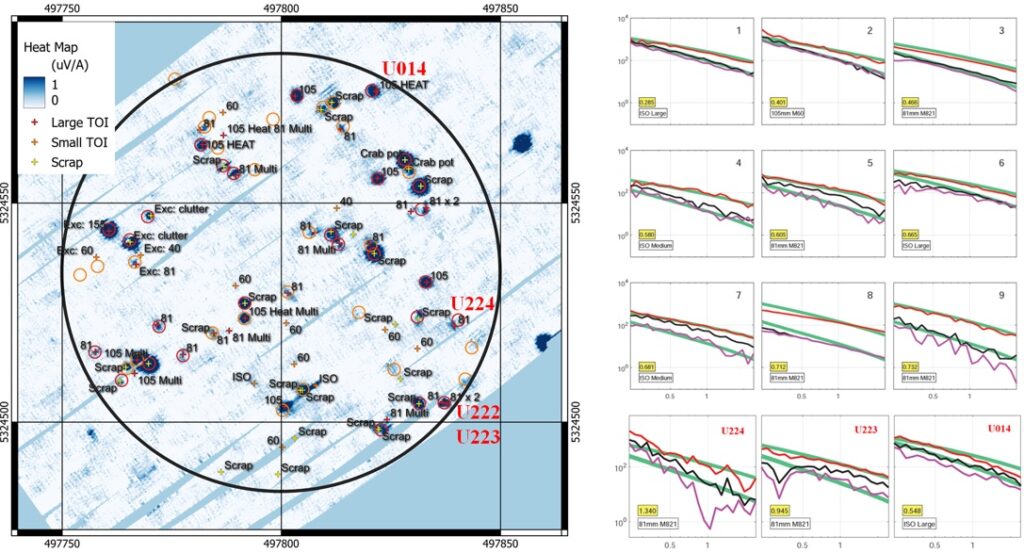
Figure 6. High altitude blind-grid test with fast-transmitter mode (4F). Left: heat-map of the mid time-channel and target list. The items marked with “Exc” were dragged out of the survey area and were not used for scoring. Red circles correspond to dig-decisions and orange circles to no-digs. Top-right: nine recovered polarizabilities of early digs. Bottom: recovered polarizabilities of three TOIs of U224, U223, and U014.

It is interesting to look at the three individual classification cases related to targets U224, U222/U223, and U014, which also are annotated near their locations in the heat map. Recall we discussed the use of the SA method to boost signals for detection. The SA example with high altitude data is shown in Figure 3. Using the SA response, we picked the two targets. One of the targets correctly classified as TOI is U224 (81mm) despite its noisy recovered polarizabilities shown in the bottom row of Figure 6. In our section on inversion, we discussed the case in which two objects U222 (81mm) and U223 (81mm) were closely spaced, and their polarizabilities were recovered accurately for low altitude data. However, for the high-altitude data, only U223 (its recovered polarizabilities shown in the middle plot of the bottom row of Figure 6) was correctly detected and classified. U222 failed to resolve. Another large item listed in Figure 6 is U014 (105mm HEAT). The item was correctly classified as TOI, and the prediction of UXO type is ISO large according to the best polarizability match. For the same item, we will show that the low altitude data allow predicting a more accurate classification result.

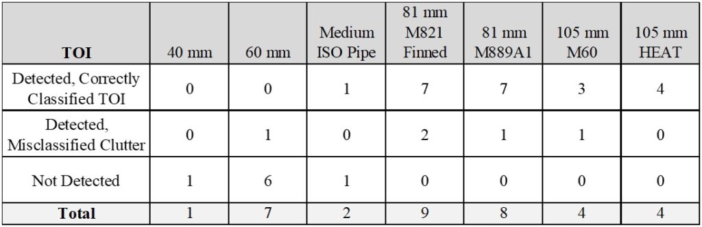
At this high-altitude survey, none of the TOI smaller than an 81mm mortar has a corresponding detection in the target list submitted to IDA. The detection and classification performance at the selected operating point is listed in Table 1.

Table 1. IDA generated scoring results for the high-altitude fast base-frequency at the selected operating point.

Performance at low altitude

At low altitude (0.5 to 0.75m), a map of the UltraTEM data collected with the fast base-frequency (4F) is shown in Figure 7. The map is annotated with the ground-truth designations of the closest item to each predicted target. Within the IDA determined radius of 3.5m, all TOI have a corresponding target pick which means that the probability of detection is 1.0. Same as the fast base-frequency (4F) data, the probability of detection is 1 for the slow base-frequency (4D) data (the corresponding map is not shown due to the limited space).

Figure 7. Low altitude blind-grid test with fast-transmitter mode (4F). Left: heat-map of the tmid time-channel and target list. Each anomaly is described from the closest item in the ground-truth provided by IDA. The items marked with “Exc” were dragged out of the survey area and were not used for scoring. Top right: nine recovered polarizabilities of early digs. Bottom: recovered polarizabilities of three 60mm grenades and one 40mm shell.

As a comparison with the high-altitude case, the top-right panel of Figure 7 presents the polarizabilities of a few top-ranked digs for the low altitude data. In contrast to those in Figure 6, the polarizabilities recovered over the 9 targets have excellent matches (highlighted in yellow) to the library ones. In fact, the polarizabilities for all targets, including the 40mm projectile and 60mm mortar (the bottom row of Figure 7), are good matches to the library polarizabilities. Overall, all have L123 match corresponding to targets of interest meeting the performance objective of 0.5. The same performance polarizability match is also achieved for slow transmitter base-frequency (4D) data (Billings et al, 2023). In Figure 7, the two polarizability plots are annotated for targets U224 (81mm) and U014 (105mm HEAT). As compared with the two annotated in Figure 6, the UXO types are correctly predicted for the low altitude data, with library matches of 0.043 and 0.099, respectively.

As an accurate recovery of polarizabilities is achieved for the low altitude data, it is equally important to examine the estimate of target locations. To check the location accuracy, we computed offsets between predicted and the “ground-truth” positions for the low-altitude slow frequency 4D and fast frequency 4F data. Upon some adjustments to WGS-84 coordinates used by PNNL (i.e., a 1.53m correction to the Easting coordinate and a 0.27m correction the Northing coordinate, Billings et al, 2023), Figure 8 (a) shows the corrected offsets where many of the slow frequency 4D and fast frequency 4F positions fall with 50cm range. Only two items in the fast frequency 4F data (in black circles) and four items (in red circles) in the slow frequency 4D data have a residual positional error of greater than 50cm. In addition, Figure 8 (b) shows the relative difference between the slow frequency 4D and fast frequency 4F derived positions. None has a relative difference of greater than 50cm. Given the uncertainties in the positions of both the PNNL ground-truth (which incidentally only provided to within the nearest 10cm) and the good match between the positions derived from the slow frequency 4D and fast frequency 4F datasets, we believe that the location accuracy of inverted positions obtained from the UltraTEM data well meets the objective: i.e., for 90% of inverted positions to be closer than 50cm to the “true” positions.

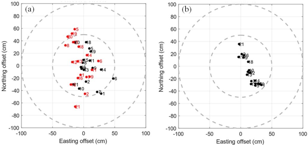
Figure 8. Positions derived from the UltraTEMA-4 platform relative to the PNNL supplied ground-truth. (a) Offsets of 4F and 4D. (b) Location difference between 4F and 4D.

As a summary of the classification performance, Figure 9 shows the receiver operating characteristic curves (ROC) for both the slow and fast-transmitter base frequency data. For the fast frequency 4F data, there are five false positives at demonstrator threshold and only two false positives at best threshold. For the slow frequency 4D data, there are six false positives at demonstrator threshold and only three false positives at best threshold. All TOIs were correctly classified for both data sets. The classification objective has been achieved for both low-altitude datasets: the probability of classification of both dig-lists is one.

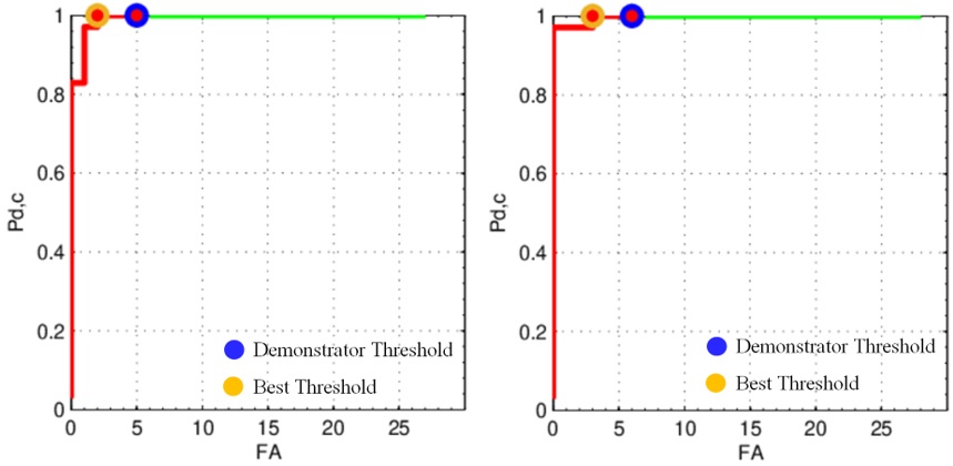
Figure 9. Receiver operating curves of low altitude data: (a) Fast transmitter mode. (b) Slow transmitter mode.

Conclusions

This paper presents the works performed under SERDP MR19-126 and ESTCP MR19-5073 that aim to address the challenges arising from underwater munitions detection and characterization. These challenges are technical and operational, including the effects of conductive seawater on the measured target response and the suitable signal model for processing, the maintenance of sensor positional accuracy for achieving a full surveying coverage, and a stable control of surveying altitude for obtaining sufficient SNR.

In the technical aspects, we have developed a full integral equation technique to model and characterize EMI responses in a multi-layered medium. To mitigate the influence of inaccurate sensor positioning on a recovery of the polarizabilities of a target, we have proposed the modified inversion methods that implicitly and explicitly account for sensor positioning errors. To increase detectability at large standoffs, a synthetic aperture method has been attempted to boost target signals.

In the operational and instrument development aspects, the UltraTEM has had several modifications and improvements in hardware and software. At present, the system is equipped with unique features, including: (1) large transmitter coils and high transmitter dipole moment (e.g., 300 Amp turns for the marine UltraTEM); (2) configurability for multiple transmitter loops and sensor cubes to address specific applications and environments; (3) extremely rugged and reliable electronics with precision time synchronization; and (4) integration with BTField software, which can be easily configured for new transmitter receiver geometries and can be used for near real-time processing and interpretation of data. By combining these with the results of demonstration of blind test at Sequim Bay, we can draw the following conclusions:

• Within the time range of interest, the dipole signal model used in terrestrial EMI sensing can be effectively utilized for marine detection and characterization.
• Conductive background responses, which can obscure or distort target responses, can be effectively removed by modeling the marine environment as a layered structure or with a properly designed high-pass filter.
• Accounting for errors in sensor positioning is important to accurately recover the polarizabilties of a target through inversion. The IMLI and JETSP methods serve the purpose well.
• Detection of weak targets can be enhanced via the synthetic aperture method that optimally stacks multiple transmitter–receiver measured responses.
• Multiple surveys at 0.5m to 1.5m+ altitude above the sea-bottom demonstrated that the UltraTEM tow-fish is stable to track the sea-bottom profile without significant changes in platform pitch and roll and without large excursions from the intended track. The low-altitude data collected at the fast-transmitter frequency (4F) achieved 100% coverage of the Blind-Grid area. At small standoff distance (0.5 to 0.75m) to the seafloor, we expect the UltraTEM system will allow for collection of high SNR data for production of underwater UXO surveys.
• For each of the two low-altitude blind-grid submissions, all seeded targets have a corresponding target pick which means that the probability of detection is 1.0. The receiver operating characteristic curves (ROC) show that both low-altitude submissions achieve the probability of classification of 1.0 with five or six false positives at demonstrator threshold and only two or three false positives at the best threshold. The location accuracy of the classified targets, as compared to the ground-truth positions, is within 50cm. We have demonstrated that AGC is feasible within the marine environment in situations where the tow-fish can be operated at low altitude (e.g., ~ 0.5m) above the bottom.

Acknowledgements

The authors would like to thank Steve Saville for coordinating review process and providing constructive edits that help improve the manuscript. This work is supported by the SERDP project MR19-1261 and ESTCP MR19-5073.

References

Pasion, L. and Oldenburg, D. W., 2001, A discrimination algorithm for UXO using time domain electromagnetics. Journal of Engineering and Environmental Geophysics, 28, no. 2, p. 91-102.
Bell, T., Barrow, B. Miller, J., 2001, Subsurface discrimination using electromagnetic induction sensors: IEEE Transactions Geoscience and Remote Sensing, v39, p.1286–1293.
Shubitidze F., EMI modeling for UXO detection and discrimination underwater, SERDP MM1632, 2011.
Schultz, G., Shubitidze, F., Miller, J., and Evans, R., 2011, Active source electromagnetic methods for marine munitions: Proceedings of SPIE, Vol. 8017
Bell T., Barrow B., Steinhurst D, Harbaugh G., Friedrichs C., and Massey G., Empirical investigation of the factors influencing marine applications of EMI, SERDP MR2409, 2016.
Billings S., and Song L.-P., Determining Detection and Classification Potential of Munitions using Advanced EMI Sensors in the Underwater Environment, SERDP Project MR-2412. 2016
Billings, S. D., Funk, R. J., Gamey, J., 2023, UltraTEM Marine towed system for detection and characterization of buried ordnance: ESTCP MR19-5073, report.
Billings, S. D., Song, L.-P., 2020, Advanced marine EMI processing techniques for munitions detection and classification: SERDP MR19-1261, interim report.
Song, L.-P., S. D. Billings, L. R. Pasion, and Douglas W. Oldenburg, Transient electromagnetic scattering of a metallic object buried in underwater sediments, IEEE Trans. Geoscience and Remote Sensing, 54 (2), 1091-1102, 2016.
Knaak, A., Snieder, R., Súilleabháin, L.O., Fan, Y., and Ramirez-Mejia, D., 2015, Optimized 3D synthetic aperture for controlled-source electromagnetics: Geophysics, v. 80, no. 6, E309–E316.
Song L.-P., and Billings S., 2023, Synthetic aperture method for enhancing detectability in transient electromagnetic induction sensing of underwater munitions: in preparation.
Song, L.-P., Pasion, L. R., Billings, S. D., and Oldenburg, D. W., 2011, Nonlinear inversion for multiple objects in transient electromagnetic induction sensing of unexploded ordnance: technique and applications: IEEE TGRS, v.49, no. 10, p. 4007–4020.
Pasion, L. R. and Song, L.-P., 2021, Strategies and methods for Effective UXO Classification: SERDP MR-2318, report.
Song, L.-P., Sinex, D., Billings, S. D., 2023, Inversion in transient electromagnetic induction sensing of underwater metallic munitions with sensor positioning errors: SERDP MR19-1261, report.

Author Bios