
Remke L. van Dam
Greg Maude
Graham Jenke
Andrew Duncan
Peter K. Fullagar
Abstract
Loupe TEM is a new transient electromagnetic profiling system for efficient mapping of near-surface ground conductivity. The system is operated by a two-person crew who carry the transmitter coil and 3-component receiver coils on backpacks. Benefits of the system include the high productivity compared to traditional moving-loop EM and the ability to survey in various types of terrain and through dense vegetation. We used the Loupe TEM system in mid-2020 in the Pilbara region of Western Australia to investigate potential fluid pathways and contamination around an overflow pond. A total of 23.5 line kilometres of data was acquired in two days on a dense grid with 20 m line spacing. We used a 75 Hz base frequency and stacked 300 transients to improve the signal-to-noise ratio. Data were gridded to show spatial features and modelled to create conductivity depth images. Supporting information included a frequency-domain EM survey using a Geonics EM-34 system, passive seismic data obtained using the Sara GeoBox, and information from groundwater monitoring bores. The results identified various laterally coherent zones with elevated electrical conductivities, some of which appeared to originate from the pond. Features of interest included a shallow clay layer, a likely bedrock shear zone, and possible contamination. The Loupe TEM data correlated well with EM-34 bulk conductivity values, while passive seismic data provided useful supplementary information on bedrock depth.
Introduction
Electromagnetic (EM) and electrical geophysical methods are frequently used for environmental and hydrogeological investigations thanks to their ability to investigate electrical conductivity variations induced by textural, soil wetness, and fluid salinity differences. Possible applications include groundwater studies, managed aquifer recharge, dam seepage mapping, structural mapping, shallow conductor exploration, saline intrusion assessment, and others.
When conducting site investigations using geophysical methods, one often needs to find a trade-off between depth of investigation, detail of information, and survey efficiency. Direct-current electrical resistivity imaging or tomography (ERI/ERT) methods allow for creating models of the subsurface resistivity distribution with a considerable amount of detail and good depth of investigation. However, data collection is relatively slow, making it tedious for larger-scale site investigations.
Frequency-domain EM (FDEM) systems collect continuous-mode data without ground contact, but the resulting bulk electrical conductivity data offer limited depth information. FDEM systems that use multiple or variable loop orientations and separations are often either rather inefficient or challenging to operate due to their large weight.
Time-domain EM (or transient EM, TEM) methods afford good depths of investigation and can be used to create models of the subsurface conductivity distribution. However, the standard ground-based moving loop approach is relatively inefficient. Airborne systems on the other hand have high operational costs and are not suitable for all applications (Behroozmand et al., 2019).
To improve efficiency of TEM data acquisition, various ground-based transient EM profiling systems have been developed in recent years, including nanoTEM, agTEM, and tTEM (e.g, Hatch et al., 2010; Allen, 2019; Auken et al., 2019). These systems can achieve a good productivity and significant depths of investigation. However, as these systems are typically towed behind a regular or all-terrain vehicle, their use is mostly limited to tracks and some agricultural fields. The Loupe TEM system, used in our work, is highly mobile and can go virtually anywhere where a person can walk.
In this article, we describe the Loupe TEM system, including the design, instrument and loop details, and standard processing procedures. We then present results of a recent case study, where we used Loupe for an environmental site investigation. We discuss the objective, instrument configuration, survey design, data processing and modelling, and results.
Loupe TEM
System details
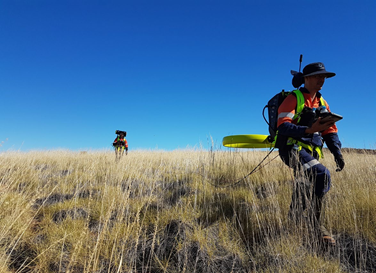
Loupe is a new portable time-domain electromagnetic (TDEM) profiling system, with the transmitter and receiver carried by separate operators and joined by a cable (Figure 1). With the weight centred behind the operators on ergonomically designed backpacks, the equipment is easy to carry and operate. The system is designed to be used in continuous profiling mode with a variable transmitter-receiver separation (Street et al., 2018). Datalogging and track guidance is handled by a field tablet that is wirelessly connected to the data acquisition system in the transmitter backpack.
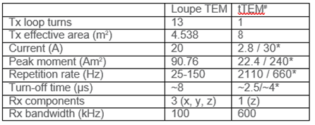
The most recent version of the system has a transmitter (Tx) coil with 13 turns with a diameter of 667 mm. With a current of 20 A, the Tx has a maximum moment of 90.76 Am2 (Table 1). The Tx operates at selectable base frequencies from 25 to 150 Hz. It uses a 50% duty cycle and produces a bi-polar square waveform, switching off in 8 microseconds. At the standard Tx repetition rate of 75 Hz, one full cycle of the transmitter waveform (plus, zero, minus, zero) takes 13.33 ms.
The receiver (Rx) is a 3-axis coil with a common centre point and effective areas (after amplification) of 200 m2 (Duncan and Street, 2019). The Rx sensor has a 100 kHz bandwidth using a sampling rate up to 504 kHz. Receiver gain can be varied depending on transmitter-receiver separation. Signal voltages are recorded and processed to 22 logarithmically spaced time windows, to around 2.7 milliseconds (ms) after signal shutoff for the 75 Hz transmitter base frequency. Table 1 compares the specifications of Loupe with recently published information on the tTEM system (Auken et al., 2019).
The maximum depth of investigation (DOI) of TEM systems
is proportional to the transmitter current strength, the area of the Tx loop, and the resistivity of the ground, and inversely proportional to system and random noise (e.g., Flores et al., 2013) or the square root of the number of transients in a stack (Auken et al., 2019). Compared to the tTEM system, which has a DOI of 60-70 m in material of around 50 Ωm (Auken et al., 2019), the Loupe has 38% of the peak moment. The number of transients in a stack is also typically smaller due to the difference in repetition rate. In its current design, the receiver is connected to the transmitter backpack by means of a cable that passes analogue signals from the receiver sensor to the data acquisition electronics in the transmitter backpack. To avoid electromagnetic interference, the receiver backpack currently has no data acquisition electronics. Development aimed at placing the data acquisition unit and a second GPS antenna in the receiver operator’s backpack is ongoing; this step would remove the need for the cable tether and enable more system configurations and different applications.
Data processing
Loupe TEM data QA/QC and pre-processing typically includes the following steps. Equipment operators conduct pre-start and on-the-fly checks of GPS positioning accuracy and consistency of signal decays. The lateral coherency of the overall response can be checked both while a survey is in progress and after completion of individual or multiple lines.
After downloading the raw survey data from the instrument, data are stacked, filtered if required, and windowed. During the stacking process, noise caused by the motion of the operators is considerably attenuated. Data are then corrected for system response. The typical stack includes two seconds of data, which at a transmitter base frequency of 75 Hz, equates to 300 transients (150 full signal periods).
Stacked data are output at user-selected intervals with or without overlap between stacking windows. A common output is one reading per second. At a walking pace of 3.7 km/hr (observed raw survey speed over gently undulating terrain with occasionally dense vegetation), this results in approximately one reading per meter. The final pre-processing step is the application of a parallax correction; data is typically plotted in plan and section at a location half way between Tx and Rx – the single GPS receiver (0.5 m in front of the centre of the Tx) is used to calculate this central point.
Additional steps to improve the signal-to-noise ratio and to remove spurious readings may be beneficial or necessary, especially where surveys are conducted through dense vegetation or over steep topography. In these cases, there is more operator movement and loop orientation is more variable. Processing steps may include a larger amount of basic stacking (for example, up to 10 seconds or 1500 transients), application of a median filter to remove outliers, or smoothing of time decays.
Data visualization and modelling
Data analysis typically starts with gridding of ground response data for different times after signal shut-off to visualize the lateral variations of electrical conductivity. To obtain variations in electrical conductivity with depth, conductivity depth images (CDIs) or inversion models can be generated using appropriate software.
CDI processing is the simplest and fastest way to obtain a first-pass interpretation of the sub-surface conductivity. Depths assigned to compact conductors in CDIs can be exaggerated, but this is also a limitation of 1D inversion. The 2D assumption invoked in a 2.5D inversion is not always appropriate. The time and cost requirements associated with a full 3D inversion are considerable, though fast approximate 3D inversion could be effective for delineation of localised conductors (e.g. Fullagar and Woods, 2016).
Here, we used EmaxAir CDI software developed by Fullagar Geophysics (Fullagar and Reid, 2001). At each delay time, tn, the algorithm computes the apparent conductivity, σa, and then determines the depth to the current maximum at time tn in a half-space of conductivity σa. For dB/dt data and a square-wave transmitter waveform, the depth to the current maximum is approximately (𝑡𝑛/2 𝜇0 𝜎𝑎)0. 5. In this way n conductivity-depth pairs are generated at each station along the Loupe profile. The conductivity-depth pairs from successive stations can then be gridded to produce a CDI section for each survey line or interpolated to create an approximate 3D conductivity distribution.
For slingram configurations such as used by Loupe, the apparent conductivity of individual dB/dt components can be non-unique. However, this possible source of ambiguity can be virtually eliminated by processing the total field amplitude, |𝑑B⁄ dt|, defined as
|𝑑B⁄ dt |={(𝑑B𝑥 ⁄ dt )2+(𝑑By ⁄ dt )2+(𝑑Bz ⁄ dt )2}0. 5
(Schaa et al, 2006). The user can control the number of readings processed at each station, either by specifying a time range or by defining a noise floor. Finally, the CDIs can be “sharpened” to enhance resolution (Fullagar and Pears, 2010).
Case Study
Objectives and approach
In mid-2020, we conducted a geophysical survey at a mining operation in the Pilbara region of Western Australia to investigate the area around a geomembrane-lined facility for storage of overflow processing water during high rainfall events. The assumption was that seepage or fluids from a past overtopping might be present in bedrock fractures outside the pond area. Evaluation of existing groundwater sampling data at the site showed that seepage would likely be associated with elevated bulk electrical conductivities values. A Geonics EM-34 frequency-domain EM survey conducted several years prior had identified various areas of interest.
The primary objective of the site investigation was to map spatial and vertical variations in ground conductivity potentially caused by the presence of contaminated soils and groundwater, and by seepage in bedrock shear and fracture zones. A secondary objective was to estimate the depth to fresh bedrock. The crystalline granitic bedrock was believed to have a limited weathering profile at a depth of 3 to 5 m below a clayey or silty overburden. Overburden thickness above bedrock shear and fracture zones would possibly be greater. Open-file airborne VTEM data indicated that bedrock in the region was generally highly resistive.
Multiple monitoring bores exist at the site (Figure 2) and water sampling conducted in 2020 showed that specific conductance values ranged from around 3.5 to 45.0 mS/cm. Unfortunately, no logging data or depth to bedrock information was available for most of the bores. Additionally, since the screened intervals extended for several tens of vertical meters it was not possible to determine from what depths any possible contamination would have originated or what would have been its concentration.
The Loupe TEM profiling system was used to map spatial variations in ground conductivity at a high spatial resolution. We collected Loupe TEM data on a dense grid with a line spacing of 20 m (Figure 2). The transmitter-receiver separation was kept at approximately 12 m (using a distance rope) for the
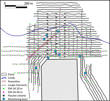
duration of the survey. We used a pulse repetition rate of 75 Hz. The signal was recorded in 22 logarithmically spaced time channels with the first and last at 0.006 and 2.27 ms from the end of the ramp, respectively. In total, 23.5 line kilometres of Loupe TEM data was acquired in 2 days. Parts of the site were heavily vegetated, but apart from occasional small detours, the Loupe survey lines could be completed as planned. The site was generally flat, except for some topography near the edges of the grid, as well as steep banks of the (dry) creek bed.
Complementary passive seismic data for depth-to-bedrock estimates were collected at 39 survey stations (Figure 2). When a strong impedance contrast is present in the subsurface, for example at the bedrock transition, the vertical and horizontal components of the ambient noise field in the overburden will differ. By converting a time series of ground motion to the frequency domain and calculating the horizontal-to-vertical spectral ratio (HVSR), the resultant resonance frequency can be related to depth of the contrast (e.g., Lane et al., 2008; Thabet, 2019). We used 3-component Geobox seismometers from SARA Electronic Instruments to acquire 10-minute time series at each station and processed the data using SARA’s GeoExplorer software.
Several years before the most recent site visit, in mid-2012, a geophysical survey was conducted using a Geonics EM-34 frequency-domain EM system. During 4 days, data were acquired using 20 and 40 m loop separations, both in a vertical co-planar loop orientation (horizontal dipoles) at 430 and 413 stations, respectively, and in a horizontal co-planar orientation at a subset of 218 and 217 stations, respectively (Figure 2). Operating frequency was 1.6 kHz and 0.4 kHz for the 20 and 40 m loop separations, respectively. Station spacing was 20 m while line spacing was approximately 40 m.
d) have Loupe transect locations overlain for reference.
Results
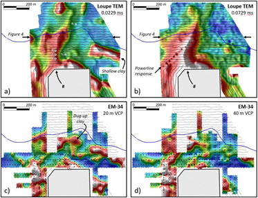
The Loupe survey data had consistent decays and showed strong lateral coherence (Figure 3a,b). Several areas with elevated ground response are present and are indicative of cultural features (e.g, the power line, visible at later times), higher soil electrical conductivities, increased overburden thickness (possibly related to bedrock fracture zones), or other features of natural and geological origin.
In many cases, the main areas of elevated signal response in the Loupe TEM data correlate very well with the EM-34 survey conducted in 2012 (Figure 3c,d). The powerline response is also clearly visible in the EM-34 data, in particular the readings with 40 m loop separation (Figure 3d). The observed differences between the EM-34 and Loupe results are partly related to the density at which data were acquired. Whereas one anomalous EM-34 data point would affect the gridded results, the much higher data density achieved using Loupe will reduce the effect of any outliers and result in a smoother gridding result.
A zone of shallow clay is clearly visible towards the right in Loupe’s early time channels (Figure 3a) but is absent from later ones (Figure 3b), supporting the interpretation of a shallow conductive feature. The EM-34 data identified this feature in readings taken with the VCP orientation at 20 m separation, which have a depth of investigation of around 15 m. In the readings at 40 m separation (depth of investigation around 30 m), the signature had significantly weakened, although the survey direction may have been a factor. Some of this clay was dug up subsequently for use as lining material when upgrading the overflow pond; it is visible in the EM-34 data (Figure 3c), but not in any of the Loupe TEM time channels.
Several of the areas with elevated signal response abut or are connected to the pond. Without supporting information, it
is not possible to conclusively attribute these to overburden thickness variations, different soil properties, or the presence of contaminated fluids. However, one strong feature in the Loupe data was not present in similar form during the 2012 EM-34 survey. This feature starts near the top left corner of the pond and extends to (and across) the creek. It has a strong signature and remains visible to at least 1.3 ms after signal shutoff (time channel 12). In 2012, the area near the creek had higher conductivity values, but there was no connection with the pond. The development of this connection suggests that one or more overtopping events in intervening years caused migration of contaminated fluids from the pond toward the creek, possibly in a bedrock shear zone.
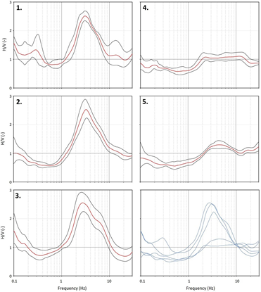
Passive seismic data from the left-most line contained a series of relatively low-amplitude but well-defined spectral frequency peaks (Figure 4). In most other areas clear peaks were absent, suggesting that depth to bedrock was either too shallow to record a usable signal or that the overburden to bedrock transition was too gradual. The area with clear spectral peaks coincided with a portion of the Loupe survey with elevated soil conductivities (Figure 3a). The correlation was not perfect, with some stations in the area with high conductivities recording no peak, and some stations outside that area having a broad peak. Nevertheless, these results do suggest that this zone with higher electrical conductivities (marked “#” in Figure 3a,b), might have greater depths to bedrock or a sharper acoustic impedance contrast. Most HVSR resonance peaks had frequencies of around 2.5 to 3.3 Hz. Using a typical value for shear wave velocity in dry,
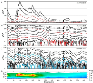
component (c). Time channels 5, 10, and 15 are coloured. The bottom panel (d) is a CDI cross section created using EmaxAir software for channels 3-13 and gridded with 1 m horizontal and 0.5 m vertical cells. A 9-point moving average filter was applied to channels 8-13.
unconsolidated material of 200 m/s (e.g., Odum et al., 2007) bedrock depth can be calculated as around 15 to 20 m below ground surface. These values are higher than expected and investigative drilling would be required to confirm these results.
Raw Loupe TEM data are shown for a survey line that shows areas with both elevated and low signal responses (Figure 5a). The small peak in channels 1 to 5 between 450 and 500 m distance (Figure 5b) is associated with the creek crossing. For the line segment from around 75 to 250 m distance, the elevated responses extend to later time channels. When plotted on a logarithmic scale, it is evident that signal decay in Z-component data is coherent to around time channel 10 (0.0729 ms) in resistive areas and channel 12 (0.1333 ms) in conductive areas (Figure 5b). At amplitudes below around 1 μV/A the random noise increases significantly; the effect of this can be reduced by applying a low-pass filter. The horizontal X component of the data displays more noise at early time channels. This is likely a result of the smaller signal amplitudes and significant noise sources on horizontal component data.
The Loupe TEM data were processed using EmaxAir software to create CDIs. Example results of this transformation using the total field data are shown in Figure 5d. The zones of elevated electrical conductivity are clearly visible, with electrical conductivities up to around 100 mS/m. The conductive features correspond to confirmed locations of high-conductivity groundwater, with specific conductance values up to around 41 mS/cm recorded around the time of the Loupe survey. However, the monitoring bores are screened over large vertical extents of 20 to 50 m and no information about the stratigraphy or depth to bedrock was available. It is therefore difficult to use these data for a more quantitative comparison with the geophysical results.
Conclusions
Profiling TEM systems allow for improved efficiencies in shallow conductivity mapping by using higher acquisition speeds while collecting feature-rich datasets. In this article, we present the Loupe TEM profiling system, which is operated by a two-person crew who carry the equipment on backpacks. The system is highly mobile and can go virtually anywhere where a person can walk.
We used the Loupe TEM system at a mine site in the Pilbara region of Western Australia to investigate potential fluid pathways and contamination around a facility for storage of overflow processing water. We achieved a daily production of up to 12 kilometres despite, at times, dense vegetation. Data were transformed to conductivity depth images (CDIs) and compared with results from a Geonics EM-34 frequency-domain EM survey conducted several years prior.
The results identified various laterally coherent zones with elevated electrical conductivities, some of which were connected to the pond. The Loupe data showed very good correlation with the EM-34 data, including in areas where shallow clay had been confirmed to exist. One area where the Loupe TEM data differed from the EM-34 data was a feature that originated at the pond extending a few hundred meters to and across a small creek (dry during both visits). This feature is a possible bedrock shear zone and the elevated conductivities in this feature may indicate contamination as result of one or more overtopping events that would have occurred during the years in between the EM-34 and Loupe TEM surveys.
Acknowledgment
We thank Brendan Ray (SGC) for field assistance, Greg Street (Loupe Geophysics) for discussions, and our client for permission to publish results of the case study.
References
Allen, D., 2019, Groundwater applications of towed TEM in diverse geology at farm scale. ASEG Extended Abstracts, doi:10.1080/22020586.2019.12073025
Auken, E., Foged, N., Larsen, J. J., Lassen, K. V. T., Maurya, P. K., Dath, S. M., and Eiskjær, T. T., 2019, tTEM—A towed transient electromagnetic system for detailed 3D imaging of the top 70 m of the subsurface. Geophysics, v. 84, no. 1, p. E13-E22.
Behroozmand, A. A., Auken, E., and Knight, R., 2019,Assessment of managed aquifer recharge sites using a new geophysical imaging method. Vadose Zone Journal, v.18, doi:10.2136/vzj2018.10.0184.
Duncan, A. and Street, G., 2019, Noise reduction in a mobile, continuous operation TEM system – Loupe. ASEG Extended Abstracts, doi:10.1080/22020586.2019.12073218.
Hatch, M., Lawrie, K., Clarke, J., Mill, P., Heinson, G., and Munday, T., 2010, Integrating ground penetrating radar and ground-based high resolution EM to improve understanding of floodplain dynamics. ASEG Extended Abstracts, doi:10.1081/22020586.2010.12041931.
Flores, C., Romo, J. M., and Vega, M., 2013, On the estimation of the maximum depth of investigation of transient electromagnetic soundings: the case of the Vizcaino transect, Mexico. Geofísica Internacional, v. 42, no. 2, p. 159-172.
Fullagar, P. K., and Reid, J. E., 2001, Emax conductivity-depth transformation of airborne TEM data: ASEG Extended Abstract, 15th International Geophysical Conference & Exhibition, Brisbane.
Fullagar, P. K., and Woods, D., 2016, Fast 3D inversion of “total field” resistive limit TEM data: ASEG Extended Abstracts, 25th International Geophysical Conference & Exhibition, Adelaide.
Fullagar, P. K., and Pears, G. A., 2010, High resolution conductivity-depth transformation of TEM data: ASEG
Extended Abstracts, 21st International Geophysical Conference & Exhibition, Sydney.
Lane, J. W., Jr., White, E. A., Steele, G. V., and Cannia, J. C., 2008, Estimation of bedrock depth using the horizontal-to-vertical (H/V) ambient-noise seismic method. Symposium on the Application of Geophysics to Engineering and Environmental Problems, 13 p.
Odum, J. K., Williams, R. A., Stephenson, W. J., Worley, D. M., von Hillebrandt-Andrade, C., Asencio, E., Irizarry, H., and Cameron, A., 2007, Near-surface shear wave velocity versus depth profiles, Vs30, and NEHRP classifications for 27 Sites in Puerto Rico. USGS Open-File Report 2007–1174.
Schaa, R., Reid, J. E., and Fullagar, P. K., 2006, Unambiguous apparent conductivity for fixed loop transient electromagnetic data: Exploration Geophysics, 37, 348-354.
Street, G., Duncan, A., Fullagar, P., and Tresidder, R., 2018, LOUPE – a portable EM profiling system. ASEG Extended Abstracts, doi:10.1071/ASEG2018abW10_3G.
Thabet, M., 2019, Site-specific relationships between bedrock depth and HVSR fundamental resonance frequency using KiK-NET data from Japan. Pure and Applied Geophysics, v. 176, p. 4809-4831, doi:10.1007/s00024-019-02256-7.
Author Bios

Remke L. van Dam
Southern Geoscience Consultants 39 Richardson St., West Perth Western Australia 6005
Australia
Remke van Dam is a Principal Geophysicist with Southern Geoscience Consultants in Perth, Australia, where he promotes geophysical solutions for a broad range of environmental, engineering, and groundwater applications. He received his Ph.D. from VU University (2001) in Amsterdam and specializes in the use of electromagnetic and electrical geophysical methods. He has published over 30 peer-reviewed papers and has extensive field experience around the world. He is a Past President of the SEG Near-Surface Technical Section and is currently an Associate Editor of the Journal of Environmental and Engineering Geophysics.

Greg Maude
Southern Geoscience Consultants 39 Richardson St., West Perth Western Australia 6005
Australia
Greg Maude qualified with a B.Sc. in Geophysics from Curtin University in Perth and has over 20 years’ experience in geophysical exploration. He has strong expertise in acquisition, processing and modelling of EM and ground magnetic data, having spent 10 years as a geophysical operator and crew leader culminating in the establishment and running of his own acquisition company. Greg now manages a diverse portfolio of projects providing specialised geophysical support to clients in mineral exploration and for near-surface applications. He manages SGC’s in-house data acquisition and training business and is a member of SGC’s Board of Directors and senior management.

Graham Jenke
Southern Geoscience Consultants 39 Richardson St., West Perth Western Australia 6005
Australia
Graham Jenke is a geophysicist with more than forty years’ experience in mineral exploration using a variety of techniques for a variety of commodities, mainly in Australia. He has also worked extensively with hydrogeologists in water exploration and environmental monitoring, and is a member of the ASEG, AIG and SEG.

Peter Fullagar holds a Ph.D. in geophysics from UBC. He has over 35 years’ experience in exploration and mining geophysics. During the past 20 years he has consulted privately and has developed processing and inversion software primarily for electromagnetic and potential field methods. Peter is a member of ASEG, SEG and KEGS. He is currently based in Vancouver.
Andrew Duncan
Loupe Geophysics
3 The Avenue, Midland Western Australia 6056 Australia
Andrew Duncan has a B.Sc. (Hons) in geophysics from Monash University (1986) in Melbourne. In 1989, he joined Aerodata / World Geoscience in Perth where he was responsible for the technical oversight of airborne electromagnetic survey systems. In 1994, Andrew started Electromagnetic Imaging Technology Pty Ltd (EMIT) and developed, with the sponsorship and assistance of WMC Resources, the first generation of SMARTem receiver system for TEM and IP methods. Andrew has interests in electromagnetic physics and modelling and is involved in the development of the Loupe portable EM system. He has been the recipient of the ASEG’s Grahame Sands and Laric Hawkins awards.