Combining Geophysical Methods as a Tool to Improve the Quality of the Results of Hydrogeophysical Investigation Interpretations

INTRODUCTION

Combining geophysical methods has been around for quite a long time and is an independent branch of geophysics. A successful combination of methods is the key to solving various geophysical problems. Now in the era of rapid development of numerical modeling methods, geophysical methods are combined at the level of solving forward and inverse problems, i.e. at the quantitative level. Speaking about joint inverse problems, one cannot but mention the pioneering work of Vozoff in this area, in the 1980s.

In this short review article, we will discuss modern methods of joint inversion applied to hydrogeophysical problems. First, let’s define what a joint inversion is. Joint inversion is an algorithm for solving an inverse problem for two or more methods that have something in common, such as boundaries, properties, or gradients of these properties. It is also possible to consider the images of petrophysical sections (their structures) as a common parameter. It should be noted that if the sections of different petrophysical properties have nothing in common, the algorithms of joint inversion should not be applied, since they will rather worsen the result.

The use of joint inversions is a special way of incorporating a priori information, imposing some restrictions on parameters’ changes for the methods involved in the joint inversion. Application of joint criteria allows suppression of equivalence significantly, but only if, from the geological point of view, the criteria is chosen correctly. After all, the result of formal inversion is not a final solution and due to equivalence, especially in the areas of poor sensitivity of the section elements, the problem may have many, although often close, solutions.

The main goal of joint inversion is to take the best from each dataset used and use this in constructing a joint resulting model that satisfies all the methods involved in the inversion. This can be either specific boundaries or objects, or a part of the model or a range of depths.

The simplest and most natural application of joint inversion is a combination of electrical and electromagnetic methods. For example, the vertical electrical sounding (VES) and time domain electromagnetic (TDEM) methods pairing for water surveying [2] has already become classic, but we will not discuss it in this article. The results of joint use of these methods can be found in many publications for the last 30 years.

CASE EXAMPLE 1 – Joint Electrical resistivity tomography (ERT) and radio-magnetotellutics (RMT)

Another example of such a combination of methods is the joint use of radio-magnetotelluric (RMT) sounding data and ERT in a two-dimensional inverse task. This approach makes it possible to suppress equivalence significantly and improve the quality of the resulting model. The reason for this is different sensitivity of electrical and electromagnetic methods to resistive and conductive targets. Besides, the introducing of any additional joint criteria in these problems is not necessary, as these methods are joined naturally in resistivity/conductivity.

Figure 1A shows an example of a joint two-dimensional inversion of the field data of electro-tomography and RMT soundings. The two-method survey was performed to refine the geometry of the aquifer. Electrical tomography measurements were carried out with forward and reverse pole-dipole array with 5 m spacing, 2000 data points in total. The radio-magnetotelluric soundings were carried out in a single-component mode at 20 m spacing and a frequency range of 10³-10⁶ Hz. The final RMS error of fit achieved after 6 iterations was 3%. The resulting model was confirmed by a drillhole not far from the survey line.

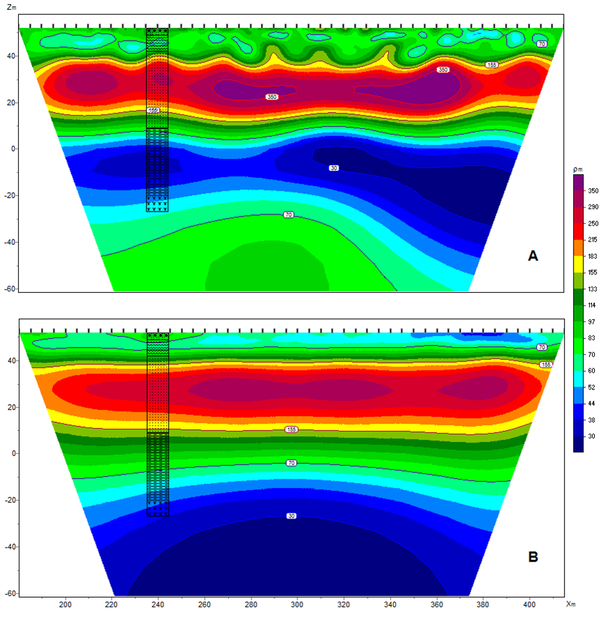
Figure 1. The result of the joint inversion of ERT and RMT data (A) and the geoelectric model based on ERT data only (B).

Figure 1B shows the result of independent ERT data inversion. By comparing the resolved models with the drillhole information, we can see the improved resolution and depth of investigation for the joint inversion result over single, ERT method model. In addition, due to suppression of equivalence, joint inversion allowed resolution of geometry of the model electrical property boundaries much more accurately.

CASE EXAMPLE 2 – Joint ERT-TDEM, ERT-seismic inversion with common layer boundaries

Next, we consider an inversion based on an arbitrary-layered model, with common layer boundaries. In this case the boundaries of the model layers are common. This approach opens more possibilities for combining geophysical methods in the inversion. For example, it is possible to combine different physical parameters (e.g., resistivity and density or velocity ) or use 1D and 2D solutions (e.g., MASW and seismic tomography) in the same task. Conversely, the concept of an arbitrary-layered media imposes restrictions on its application: the properties within the layer should not change dramatically laterally. Thus, this model is not very suitable for describing localized objects, vertical structures, etc. In the general case, the result of a joint inversion based on arbitrary layered media is a set of models for different geophysical methods with the same geometry of layer boundaries. The models obtained this way are very effective to be used as a reference at the refinement stage.

Figure 2 shows examples of joint inversion of field data within an arbitrary-layered model with common layer boundaries. The work in both cases was carried out as a part of the hydrogeological survey in order to clarify the geological section. In example 2A, electro-tomography was performed with a pole-dipole array with 10 m spacing, 700 data points in total, and TDEM soundings with coincident loops (4 stations, 40×40 m loops). The average RMS fit error of the hybrid inversion (2D+1D), was 7%. In Example 2B, dipole-dipole electro-tomography data was collected with a 1 m spacing, 400 data points in total, together with refracted-wave seismic tomography (receivers spaced at 1 m, sources were 2 m apart). The average RMS fit error of the joint two-dimensional inversion, was 3%.

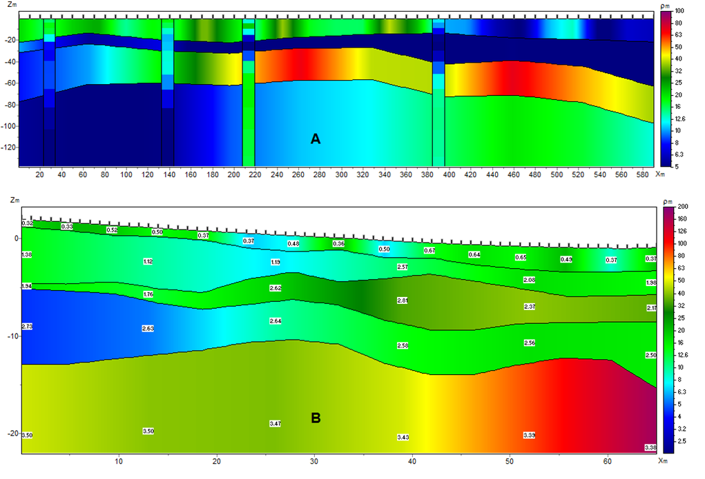
Figure 2. Results of joint inversion of electro-tomography and TDEM soundings (2A) or seismic tomography (2B) data within an arbitrary-layer model and common layer boundaries. In both sections, resistivity is indicated by color. The color-coded columns in 2A show the result of an independent 1D inversion of the TDEM data, the annotated numbers in 2B are the P-wave velocities (km/sec).

The geologic structure of the section for the examples in Figure 2 fit within the framework of an arbitrary layered model. The joint inversion helped to clarify the geological structure of the section and resolve models within a unified boundary geometry.

CASE EXAMPLE 3 – Joint inversion of ERT and seismic refraction tomography data with minimization of cross-gradients

The next group of joint inversion methods is based on minimization of additional criteria (an additional term in the objective function). The inversion in this case solves not only the problems of data misfit and model roughness minimization, but also minimizes the additional criterion responsible for the similarity of two or more models. In this review article, and specifically this case example, we will consider two main criteria: the local cross-gradient and the global common correlations

The problematic part of this approach is the need to balance the data and properties involved in the joint inversion methods. This is solved by choosing optimal normalization parameters based on sensitivity analysis of model parameters.

The cross-gradient criterion was first proposed by Meju and Gallardo [3]. It has a local behavior and is responsible for the similarity of gradient images of resolved models. The advantage of this operator in fact is that it does not force unnecessary increase of the gradients or if it causes increasing of the data misfit; instead, it relies only on the gradient of the joint model. Unfortunately, due to local properties of the operator, the algorithm still tends to produce false gradient structures if the problem is not sufficiently regularized at late iterations.

Figure 3 A and B shows an example of a joint two-dimensional cross-gradient inversion of seismic tomography (A) and electrical tomography (B) data. The joint inversion was carried out to study the hydrogeological conditions of a work area. Refracted-wave seismic tomography was performed with 5 m spacing between receivers and 10 m spacing between sources. The average RMS fit error achieved in the inversion was 4%.

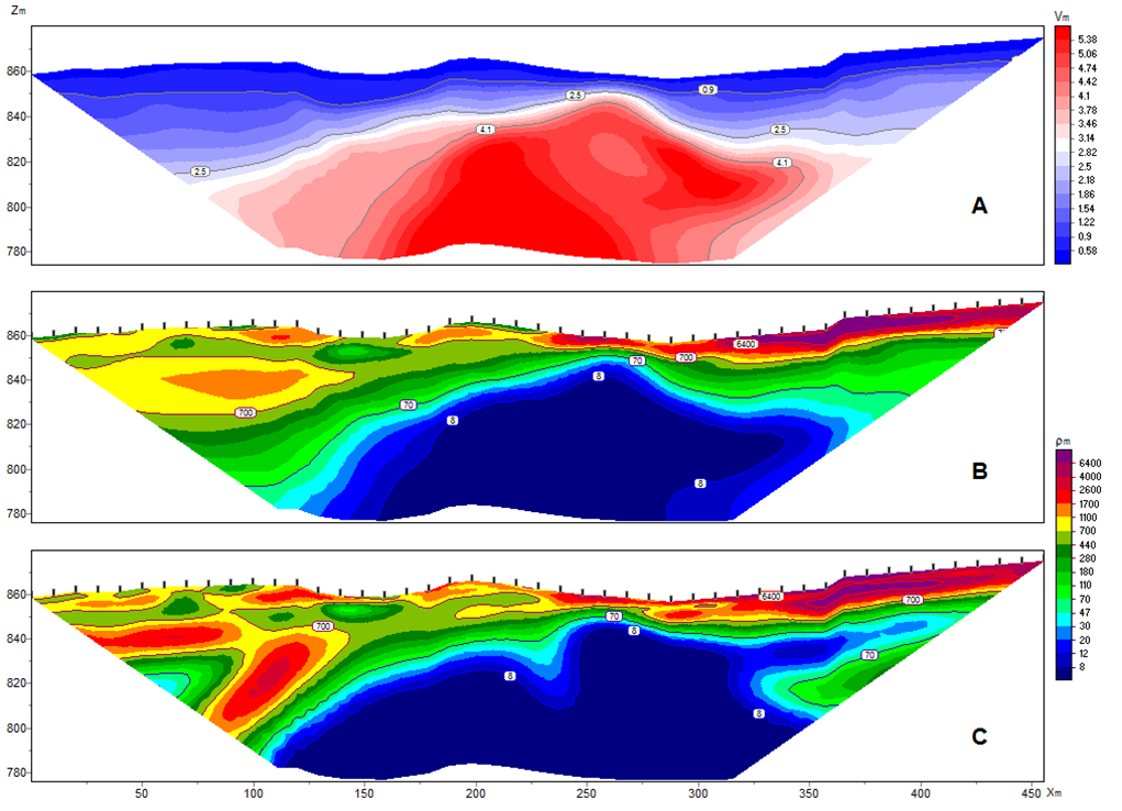
Figure 3. Results of joint inversion of seismic (3A) and electrical (3B) tomography data and geoelectric model obtained by independent inversion of electrical tomography data (3C).

Figure 3C shows the result of inversion of only the electrical tomography data. The resulting structure differs significantly from the joint inversion result because of the almost exponential decrease in sensitivity of the ERT method with depth. The joint inversion took the high-velocity boundary (in 3A) reliably detected by seismic to refine the electrical boundary (in 3B) and corrected the electrical properties in the upper part of the joint model where the electro-tomography had better resolution.

CASE EXAMPLE 4 – Joint inversion of Resistivity and Induced Polarizatio(IP) data with common correlation criterion for groundwater studies

The common correlation criterion is global and applies to the entire model rather than to its individual parts. It is a very strong interpretation tool, especially when correlations between model properties are quite strong. For example, the classical ore problem of the resistivity and IP method has a strong negative correlation of anomaly-forming object properties, whereas the seismic and gravity surveys have a good positive correlation. Because of the global impact of the operator that additionally regularizes and parameterizes the problem, the use of the algorithm, given good correlation, rarely leads to false anomalies and the solution tends to a global minimum. The nature of the correlation is chosen by the interpreter (forced version) or by the algorithm during the iteration process.

Figure 4 shows the results of joint (forced common correlation criterion) and standard inversion of ERT-IP performed to determine an aquifer’s parameters. The algorithm of forced joint inversion in this case was chosen because of inconsistency of the polarization model with the data from laboratory measurements on samples. According to the laboratory data, the resistivity and polarization data collected on samples had a predominantly negative correlation while the data (field survey apparent resistivity and IP) and the resolved models had a positive correlation.

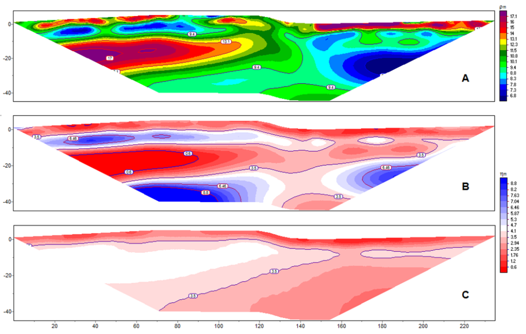
Figure 4. Results of forced joint inversion of resistivity (4A) and IP data (4B) and standard inversion of ERT-IP data (4C).

Because of the poor (compared to resistivity) sensitivity of IP (and therefore its strong equivalence), it was possible to obtain a resulting joint ERT-IP inversion model (4B) with approximately the same level of IP RMS (3%) as in the standard method of IP inversion (4C), but with a predominantly negative correlation.

GENERAL CONSIDERATIONS

It should be noted that in the joint data inversion of some methods (e.g., seismic tomography and electrical tomography) the upper two or three layers of cells are usually excluded from the 2D operator. The reason is that the near surface part of the section is generally shows different heterogeneous variations for different methods.

Our experience shows that joint inversion can be very effective for hydrogeological problems. Often it can refine the position of boundaries and significantly improve the reliability of results, where using geophysical methods separately, does not give a satisfactory result. However, the results of this joint inversion approach must be interpreted with great care, comparing the results with the models obtained separately and analysing the variation in the sizes of resolved anomalies versus the resolution capability of each individual survey method.

It should also be noted that some joint inversion algorithms usually require several inversion cycles for additional data balancing and optimal minimization settings. The quality of the result is controlled by the interpreter based on the chosen geological concept and can be improved by introducing additional a priori information (for example, by fixing or introducing known boundaries or using information about the limits of changes in the petrophysical properties of rocks).

CONCLUSION – GENERALIZED JOINT INVERSION APPROACH

So, in conclusion, the recommended general approach in combining geophysical methods and their joint inversion is as follows:

1) Selection of a set of methods to solve a geological problem based on site geology and petrophysical data. Optimal combinations of methods can be chosen based on experience and can also be found in many textbooks on general geophysics.

2) Selection of joint inversion criterion and the algorithm accordingly. Depending on geology, geometry of the boundaries, correlation of petrophysical properties and involved methods, optimal criterion can be chosen and used.

3) Introduction of a priori information. Ranges of variation of parameters, boundaries, etc can be used.

4) Cycle of joint inversion and analysis of resolved models. This cycle can be repeated several times, until a satisfactory, from the interpreter’s point of view, joint model is achieved. At the end of each cycle the inversion settings are adjusted, and the relative importance (weight) of the individual methods is changed. Each subsequent cycle may use the previous model as a starting one (used for refinement) or the original starting model.

5) At the final stage, when satisfactory results have been obtained, the model of each method can be improved using separate inversions. The model resolved in the fourth stage should be used as a reference model.

REFERENCES

1. Jupp, D. and Vozoff, K., 1975, Joint inversion of geophysical data. Geophys. J. Royal Astron. Soc. 42:977–991.
2. Leite, David Nakamura et al., 2018. Geoelectrical characterization with 1D VES/TEM joint inversion in Urupes-SP region, Paraná Basin: Applications to hydrogeology Journal of Applied Geophysics, Volume 151, p. 205-220.
3. Gallardo L. A. and Meju M. A., 2003. Characterization of heterogeneous near-surface materials by joint 2D inversion of DC resistivity and seismic data, Geophys. Res. Lett., 30, 1658.

---

Author Bios

Alex studied in Saint-Petersburg State university.  Since 2000 worked for several geophysical companies in Russia. In 2012 he founded Zond software LTD, company specializes on geophysical software development. Alex main professional interest is geophysical inversion. Author of  more than 40 publications.

Anton studied at Moscow State university.  Senior Geophysicist started at Zonge in 2008 after working at Nord West Ltd Russia for five years and achieving Bachelor of Arts in Geology and specialist in Engineering Geophysics Moscow State University. Anton specialises in supervising and processing MT survey datarvey data.