By Nathan T. Stevens1 & Stephanie R. James2
1University of Wisconsin-Madison, Department of Geoscience, Madison WI
2U.S. Geological Survey, Geology, Geophysics, and Geochemistry Science Center, Denver CO
Abstract
Changes in Earth’s cryosphere can have direct impacts on ecosystems, wildlife, and human communities that may extend to other reaches of the planet, such as through sea-level rise or altering the global carbon budget. Advances in passive seismic technology and processing methods have opened new opportunities to better understand how ice and permafrost soils are responding to changing conditions. Here, we present examples from two cryosphere applications of a simple seismic technique using horizontal-vertical spectral ratios (H/V) to explore the influences, considerations, and outcomes when applied to 1) glacial ice-thickness estimates and 2) permafrost and active-layer monitoring.
Introduction
Earth’s cold regions are experiencing unprecedented changes in climate, precipitation, and ecosystems—the long-term consequences of which are not fully understood. Estimates of ice-thicknesses provide key data for forecasting the dynamics of glaciers and ice sheets, their influence on rates of sea-level rise under warming scenarios, and the fate of water resources for mountain communities and ecosystems globally. Similarly, permafrost thaw and thermokarst (ground subsidence from melting of massive ice) significantly impact hydrologic, thermal, and biotic processes as well as the overall health and stability of aboveground plant, animal, and human communities. Knowledge of subsurface conditions beneath and within glaciers, ice, and rock is critical to understanding how Earth’s cryosphere is responding to changing climatic conditions, yet low-impact subsurface measurement capabilities offering high temporal and spatial resolution remain limited.
Geophysical techniques are uniquely positioned to provide non-invasive characterization and monitoring of physical properties below Earth’s surface across a range of scales. The recent boom in nodal seismic sensor technology and passive seismic methods have unlocked new opportunities for quick and modular seismic deployments in remote and rugged terrain. Here, we present best practices for nodal seismic deployment and processing approaches for the horizontal-vertical spectral ratio (H/V) technique, and we present demonstrations of H/V applications to 1) estimate glacier thickness on Saskatchewan Glacier, Alberta, Canada, and 2) monitor seasonal freeze/thaw dynamics and soil moisture at a lowland thermokarst site in Interior Alaska. These results demonstrate the great potential of passive seismic methods for addressing pressing questions across the cryosphere and highlight instrumental limitations that can be pushed in this pursuit.
Methods
H/V is a simple processing technique applied to three-component seismic records from individual stations used for both one-dimensional characterization and temporal monitoring. The H/V technique was initiated by Nakamura (1989) and has largely been used for microzonation studies, mapping shallow sediment layers and depth to bedrock (e.g., Bonnefoy-Claudet et al. 2006). In a layered geologic setting with strong contrasts in impedance (velocity × density) between layers, the ratio of the power spectrum between the vertical component and the average of horizontal components, termed the H/V curve. Generally, the H/V curve contains a peak at the fundamental resonance frequency, f0, that is dependent on the magnitude of the impedance contrast and the thickness of the shallower layer. Using a simple quarter-wavelength approximation, one can use the peak frequency from the H/V curve to solve for either the thickness, h, or shear-wave velocity, VS, of the shallow layer:

The cause of the H/V structure (peaks and troughs) is theorized to be the result of multiple phenomena within a complex and diffuse wavefield (García-Jerez et al. 2016). Specifically, changes in Rayleigh wave ellipticity, more or less horizontal energy from Love waves, and the resonance of body waves can each influence the H/V curve. The exact composition of the ambient wavefield is mostly unknown and transient; however, in all cases, the frequency of the fundamental peak is generally a close approximation of the fundamental shear-wave resonance frequency.
To calculate H/V, raw seismic records are minimally processed to remove uncharacteristically noisy or quiet time periods, and windowed power spectral densities (PSD) are smoothed over each channel. Then, the direct division of averaged horizontal spectra data and the vertical spectra data for time-windowed ground motion records, u(t), produce a H/V ratio as a function of frequency (f):

where uH(t) and uV(t) are the horizontal and vertical records, respectively.
Glacier Geometry Characterization
Although glacier thicknesses can be accurately constrained with in situ, active-source geophysical techniques or drilling campaigns, these tend to have large logistical requirements that limit their application to accessible and critical regions of the cryosphere (see discussion in Picotti et al., 2017). Conversely, satellite data products can be inverted for globally extensive estimates of ice thickness, but they remain subject to large errors from underlying assumptions intrinsic to the physical models employed (e.g., Farinotti et al., 2019). Demonstration of H/V as a viable tool for estimating ice thicknesses from the ambient seismic wavefield (Picotti et al., 2017) coupled with the advent of lightweight 3-C seismic sensors provide opportunities to expand in situ assessments of ice thickness with minimal equipment. Analysis by Preiswerk et al. (2018) provides site-selection guidance based on observable ice-surface features, but additional deployment and temporal considerations are necessary to fully leverage the use of H/V with new instrumentation.
Study Sites & Approach
Ideal sites should be located away from surface crevasses in sectors of a glacier with simple sub-ice topography and little to no firn—partially compacted glacier ice—or snow cover (see Preiswerk et al., 2018). These conditions are most readily found in ablation zones of mountain and outlet glaciers, near their centerlines, late in their melt seasons. Several extant on-ice deployments conform to these requirements (Figure 1.a). Here, we focus on a recent acquisition on Saskatchewan Glacier in Alberta, Canada, from August 2019 (Figure 1.b). These general acquisition timing and location requirements compete with instrument coupling as ice-surface melting rapidly degrades instrument stability. Depending on the rate of ice-surface melting, instruments can be installed in shallow boreholes that aid in preserving coupling for several days (Figure 1.c). Coupling can be further augmented by molding the base of boreholes to fit spikes on the bottom of compact seismometers using mechanical or thermal drills (Figure 1.d). Finally, frequency bands of interest for on-ice H/V analyses are shared by glacio-hydraulic processes, which can overwhelm the ambient wavefield (e.g., Nanni et al., 2020), requiring careful selection of recording times to recover clear H/V responses (peaks at f0 corresponding to ice thickness). We investigated the application of these best practices from published works for estimating ice thicknesses by conducting H/V analysis on 4 days of seismic recordings by an optimally placed Magseis/Fairfield GEN2 3-C nodal geophone on the surface of Saskatchewan Glacier. Our sampling window ran from 2019-08-07 to 2019-08-11 to encompass an instrument redeployment in a freshly prepared borehole late on 2019-08-07 and several diurnal cycles in glacier hydrology and intense ice-surface ablation, allowing inspection of the influences from variable instrument coupling and glacio-hydraulic noise on H/V results. Data were acquired at 1,000 samples per second (sps) and subsequently lowpass filtered and down sampled to 100 sps before being segmented into 1-hour blocks for H/V analysis. Blocks were subset into 30-second-long segments, rejecting those segments containing impulsive events, to produce ensembles of H/V curves, and a final representative curve, for each block using the OpenHVSR Processing Toolkit (Bignardi et al., 2018). Our analysis of these data focuses on the 1-10 Hz range, which encompasses expected values of f0 for glaciers with thicknesses of 50-500 m for typical VS of glacier ice (1850 m/s, via Equation 1). We note that the corner frequency (fc) of the nodal seismometer is 4.5 Hz, which results in a logarithmic loss of signal fidelity at frequencies below fc.
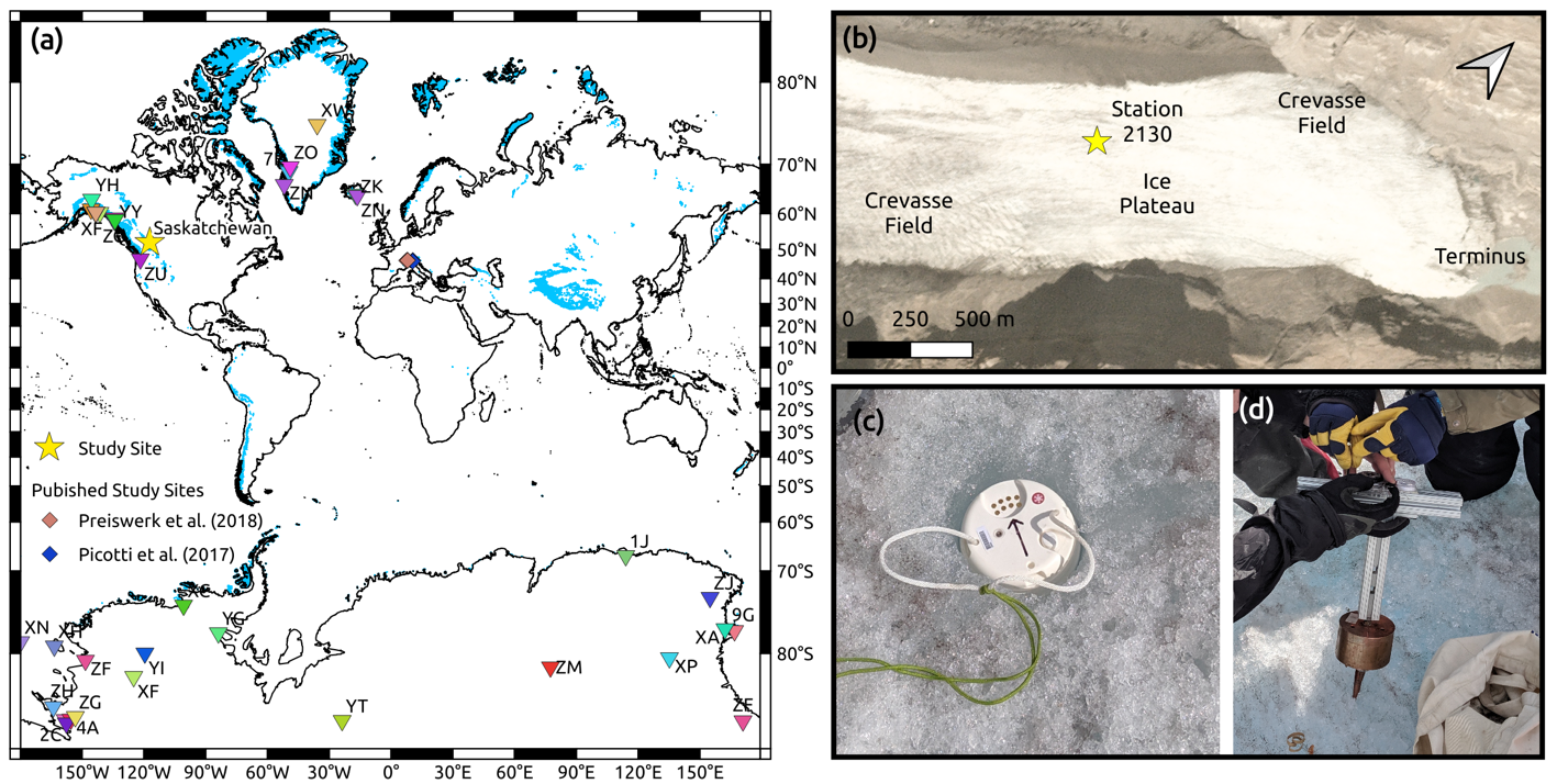
Figure 1: (a) Global map of mountain and outlet glacier locations (blue patches, Randolph Glacier Inventory v.6, Pfeffer et al., 2014) and locations of published H/V studies (diamonds), this study (star), and open-access seismic networks with on-ice deployments through the IRIS Data Management Center, https://ds.iris.edu/ds/nodes/dmc/data, (triangles, random colors). (b) Site map of the terminus of Saskatchewan Glacier and location of station 2130 relative to ice-surface features overlain on contemporary satellite imagery (Planet.com). (c) Initial installation of a node at station 2130 in a shallow borehole drilled into exposed glacier ice. The instrument top is flush with the ice surface. (d) A thermal drill used to mold borehole bases at Saskatchewan Glacier, prior to heating over a compressed gas stove. Photo credit (both): Lucas Zoet, University of Wisconsin-Madison.
Results & Discussion
We recovered consistent H/V maxima at ~2.95-3.05 Hz for the majority of the 4-day study window that were accompanied by H/V minima near 5.5 Hz (Figure 2). Ice thickness near station 2130 was estimated to be 400 m in 1952 using explosive-source seismic reflection (Meier et al., 1954). Between 1952 and 2019, the ice surface lowered by ~250 m, based upon updated GPS surveying of the ice surface at the same sites. Glacier erosion rates rarely exceed 5 cm/yr, falling well below measurement accuracy even for this length of time. Therefore, after accounting for the 67 years of ice-surface lowering, the modern ice-thickness estimate is 150 m. Using Equation 1 and a typical value of VS for temperate glacier ice (1850 m/s), this independent estimate of h corresponds to f0 = 3.08 Hz, which is consistent with values recovered from H/V analysis for much of the record. This well-defined peak is below the corner frequency of the instrument (4.5 Hz) and demonstrates that it is possible to recover reliable H/V results below this instrument-specific limit. However, this limit may still prevent H/V peak recovery at lower frequencies associated with larger ice masses (e.g., ice sheets) with similar short-period instruments.
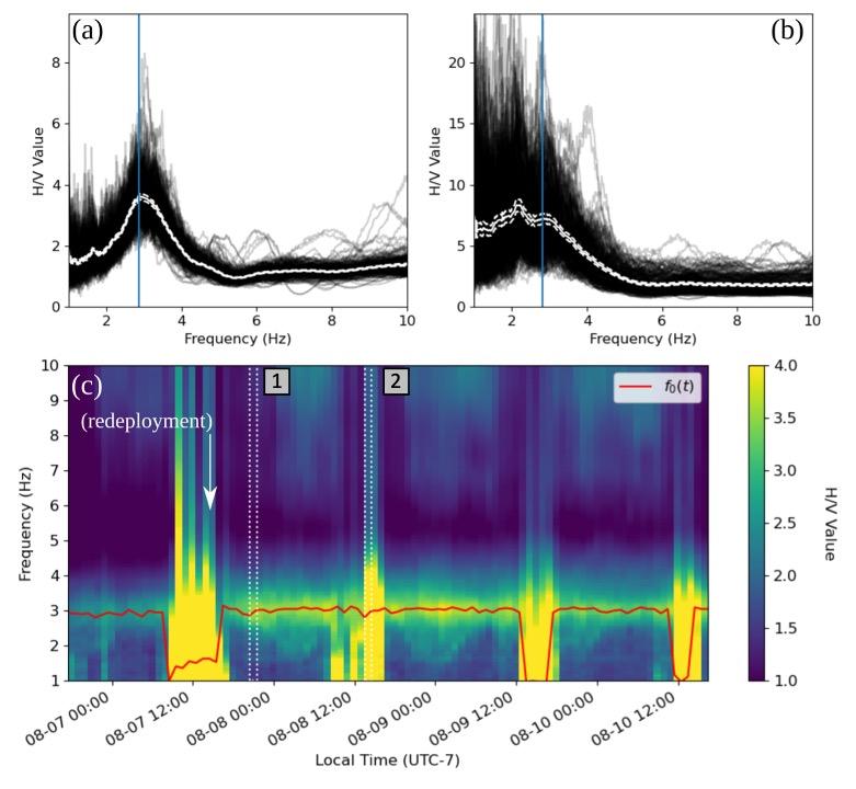
Figure 2: H/V curves from station 2130 during (a) a hydrologically quiet period—#1 in (c)—and (b) a hydrologically noisy period—#2 in (c). Mean and 95% confidence bounds (white, solid & dashed, respectively) are shown for each collection of H/V curves (black), and manually picked values of f0 are shown (blue). (c) Time-series of mean H/V curves between 2019-08-07 and 2019-08-11 with the example curve time windows shown (white dashes, 1: (a) and 2: (b)) and manually picked f0 values through time shown as a trend line (red).
The recovered ~3 Hz H/V peaks are obfuscated between 10:00 and 18:00 daily by high H/V values at low frequencies (Figure 2.b-c). These correspond with peak daily air temperatures that drive ice-surface melting and likely arise from higher glacio-hydraulic noise levels from water flowing atop, within, and beneath the glacier. Results in Figure 2 indicate that interpretable H/V responses can be recovered outside of these noisy periods, and peaks were well defined outside of peak melting periods each day. Inspection of H/V peak amplitudes (Figure 2.c) shows diminished values prior to instrument redeployment in a fresh borehole on the afternoon of 2019-08-07. Similarly, H/V peak amplitudes degraded over the subsequent 3 days with a notable decline on the 3rd day following redeployment. This is consistent with observed melt-out patterns from the field, where nodes became exposed after 3-4 days of surface melting, likely representing a nonlinear progression of instrument decoupling. Nonetheless, recovery of the ~3 Hz peak persisted even with degraded coupling during 2019-08-07 and 2019-08-10.
These results illustrate that ice thicknesses can be recovered in optimal field settings (a relatively flat, crevasse free segment of the glacier) with sufficient coupling support from a single nodal seismometer. While interpretable H/V results were recovered using 1-hour long record segments, careful selection of the timing of a record segment is necessary to avoid hydrologically noisy periods that swamp signals of interest. In these conditions, we show it is possible to recover H/V responses at frequencies below the instrument fc that have physical meaning.
Permafrost Monitoring
Permafrost—soils that have remained below 0°C for at least 2 consecutive years—underlie much of the northern hemisphere, with continuous coverage at the highest latitudes and transitions to discontinuous, then sporadic coverage toward the south. Yet, warming temperatures and changes in precipitation patterns have begun to significantly weaken and degrade permafrost soils (e.g., Jorgenson et al., 2001). Permafrost degradation can result in widespread ecosystem shifts and impacts to the global carbon budget as previously frozen organic carbon becomes available for microbial consumption and decomposition (e.g., Schuur et al., 2008; Turetsky et al., 2020). Permafrost can degrade slowly through deepening of the active layer—the surficial layer that freezes and thaws annually—or abruptly through thermokarst collapse.
Thawed and water-logged soils exhibit significantly slower VS compared to frozen, permafrost soils. Thus, H/V can be a simple technique for tracking active-layer dynamics (e.g., Kula et al. 2018, Köhler & Weidle, 2019). Active-layer thaw depth is typically measured intermittently through manual measurements with a frost-probe. Meanwhile, soil temperature and moisture probes provide continuous point-scale measurements; however, they may inadequately depict larger spatial variability. Since the diffuse ambient seismic wavefield contains complex interactions between both surface waves and body waves scattered throughout the subsurface from random sources, the H/V of a single station is expected to be representative of more aggregate properties of the near surface in the vicinity (<1 wavelength) of the sensor and, therefore, may be an advantageous technique for site characterization and monitoring across a range of scales. To investigate the applicability of H/V monitoring of active-layer and permafrost dynamics, such as seasonal thaw and soil moisture variation, we analyzed 1 year of passive seismic data recorded at a lowland boreal forest in Interior Alaska.
Study Site & Approach
The Alaska Peatland Experiment (APEX) study site is located ~35 km southwest of Fairbanks, AK, within the discontinuous permafrost domain. In April 2018, we installed an array of seismic stations (a mix of L28 3-C geophones and T120 broadband sensors) across a transect between stable, forested permafrost and two collapse-scar (thermokarst) bogs. Figure 3 shows an example seismic station, equipped with solar panels and a battery bank for continuous year-round observation. The seismometers were installed at the top of permafrost (~80 cm depth) to ensure stability (Figure 3.b) and recorded ground motion at 200 sps. Soil temperature and moisture probes were installed in summer 2018 at select seismic locations.
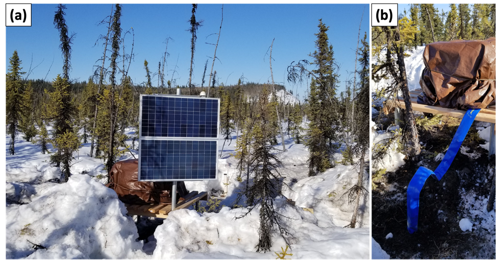
Figure 3. Seismic installation at Alaskan Peatland Experiment (APEX) study site. (a) A station box housing the data logger and battery bank, which is recharged by solar panels, located on top of a raised platform to protect the sensitive ground cover. (b) The seismometer was buried at the top of the permafrost table. Photo credit: Stephanie James, U.S. Geological Survey.
To better understand the accuracy and controls on H/V in permafrost settings, we compared timeseries of H/V curves and peak frequencies, f0, with soil temperature and moisture, focusing on the stations with collocated thermistors and soil moisture probes, for the complete monitoring year of April 2019 to April 2020. To reduce any diurnal effects, only nighttime hours (10 pm – 6 am) were used. Wind can artificially influence the H/V response (see Köhler & Weidle, 2019), which we found to be the case in our dataset. Therefore, we used wind speed data recorded at an eddy covariance tower at the site to filter out windy time periods. For this dataset, the wind speed threshold of 1.5 m/s proved suitable. Lastly, a generator was sometimes needed for other field activities, which caused a distinctive and identifiable peak in H/V around ~60 Hz; therefore, these hours were also omitted from analysis.
The hourly H/V curves were averaged into daily records, then smoothed with a 5-day rolling mean. We then picked the peak resonance frequency, f0, for each day using an automatic peak detection, then manually removed outliers. Our analysis focused on the frequency range between the fC of the L28 sensors (4.5 Hz) and the Nyquist frequency (100 Hz).
Results & Discussion
We observe a strong seasonal response in H/V amplitude and f0 (Figure 4). The frozen winter months produce flat H/V curves, often with a trough at low frequencies (<10 Hz). Peaks appear in early summer, coinciding with the rise of shallow soil temperatures above 0°C indicating thaw. H/V amplitudes increase through the summer, often reaching a maximum in early fall corresponding to maximum thaw depth (Figure 4).
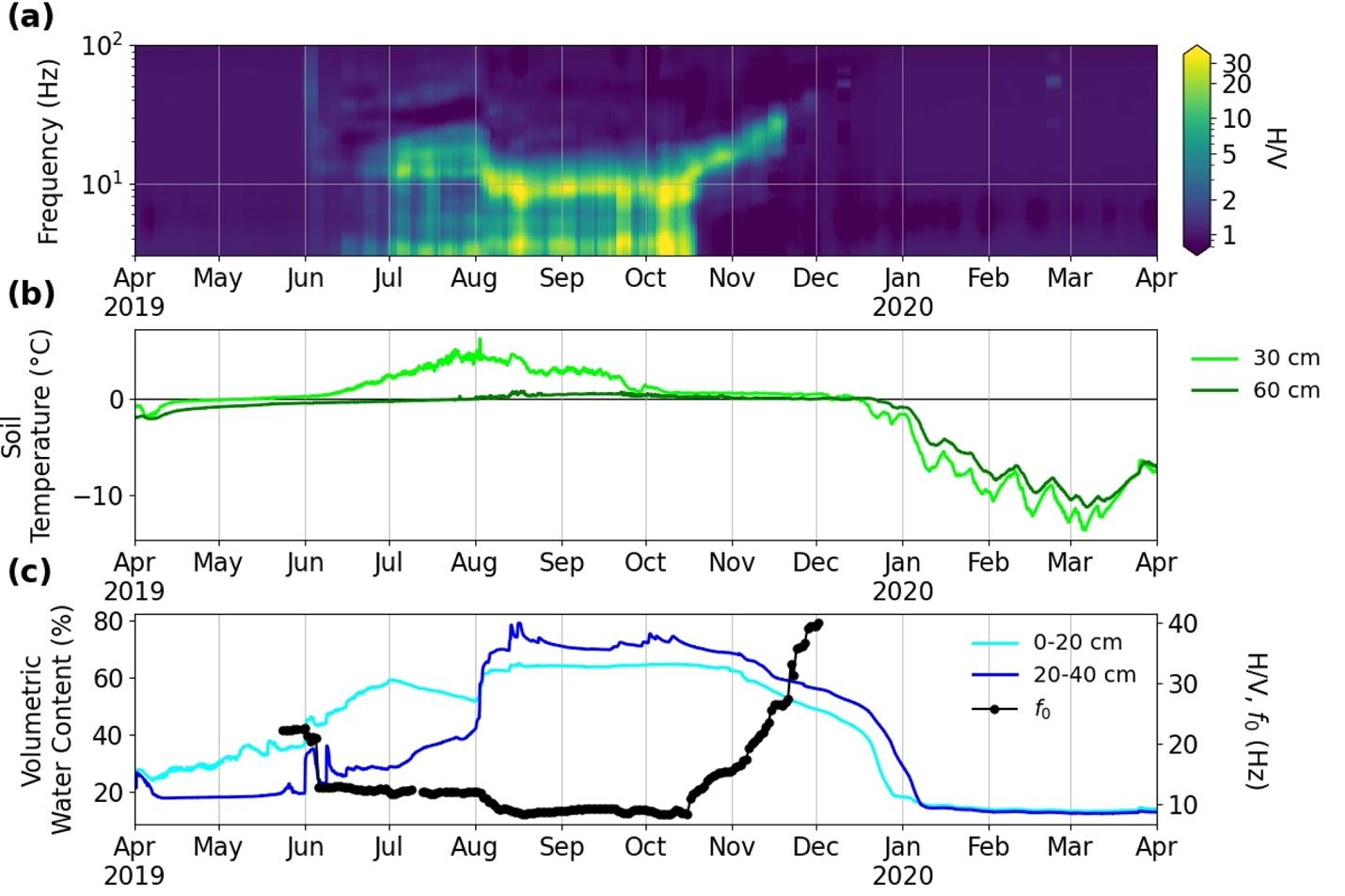
Figure 4. H/V results for a representative short-period station in stable permafrost. (a) H/V curves as a function of time (x-axis) and frequency (y-axis). Note the H/V amplitude is on a logarithmic color scale. The fundamental peak resonance frequency emerges in summer months (yellow) above the background (blue). (b) Soil temperature for 30 and 60 cm depth (light green, dark green, respectively). (c) Soil moisture from time-domain reflectometry probes, inserted at a 45° angle from 0-20 cm (light blue) and 20-40 cm depth (dark blue), in comparison to f0 picks from the H/V curves (black dots). Overall, f0 shows a clear inverse relationship to soil moisture.
The peak resonance frequency, f0, migrates to lower frequencies through the summer, from 22 Hz in May to 8.9-9.1 Hz by late summer and early fall (Figure 4c). Comparisons to soil moisture show a strong inverse relationship, where drops in f0 coincide with sharp increases in water content. Conversely, during the fall, zero-curtain time period—when latent heat from ice formation causes temperature to flatline at 0°C—soil moisture decreases correspond to sharp increases in peak frequency. The H/V response drops back to near 1 by the end of the zero-curtain period but before soil moisture is fully minimized. This is likely due to limited resolution at the high-frequency end of the spectrum as the thawed active-layer soils grew progressively thinner and became higher velocity due to ice formation. Overall, these relationships indicate thaw depth, soil moisture, and ice formation all compound to influence the H/V signature due to impacting both the VS and h of the thawed, active-layer soils. To quantitatively solve for either parameter, complementary supporting data, or reasonable assumptions on values—such as in the glacier example earlier—will be needed. Better understanding of the complexity of relationships influencing the H/V response would enable more direct and quantitative tracking of subsurface conditions with this method.
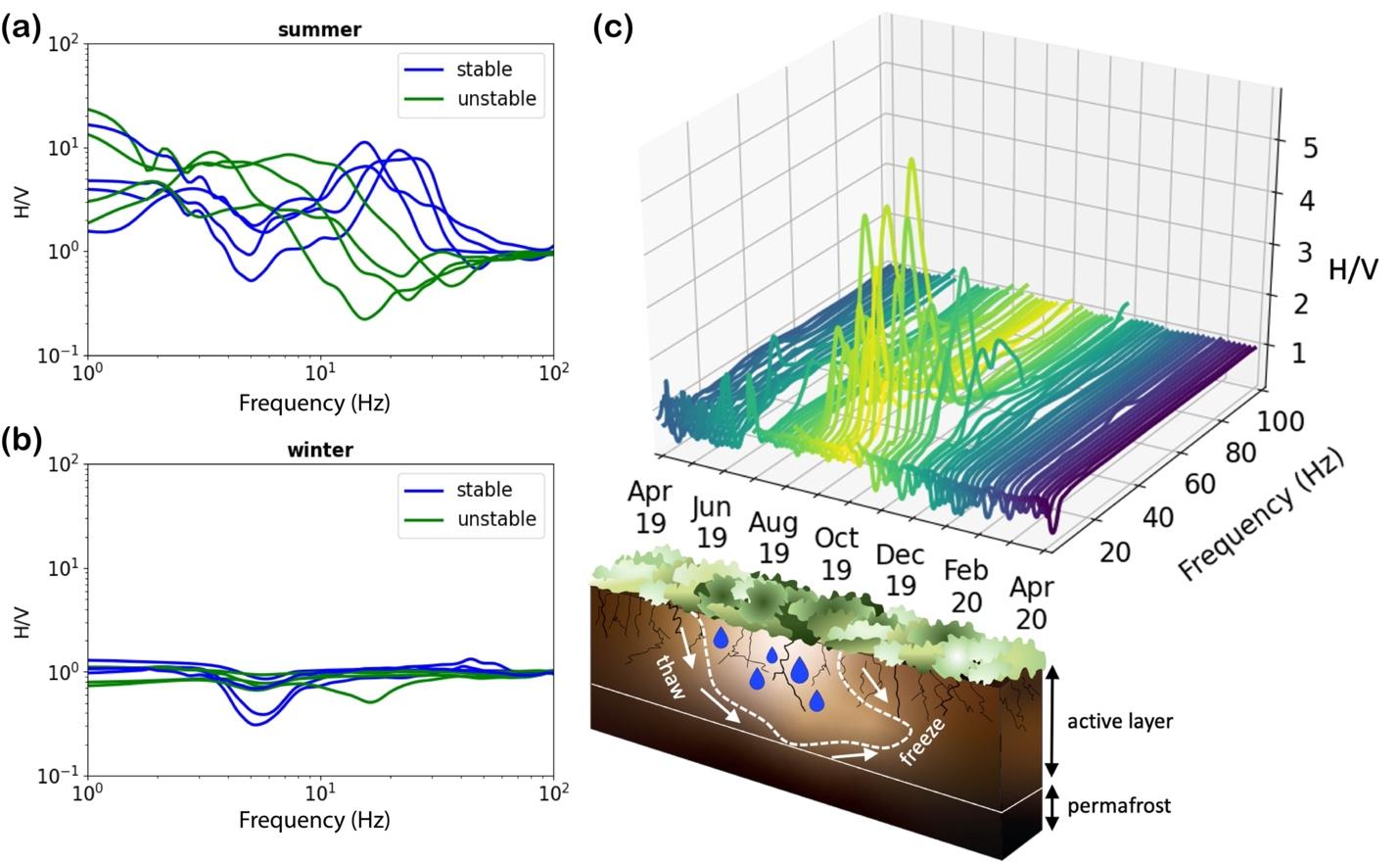
Figure 5. H/V signatures for stable (blue) and unstable (green) locations are compared for (a) summer and (b) winter seasons. (c) An example H/V time series is shown with a conceptual model of the H/V seasonal response. H/V peaks start in early summer as thaw begins. The peaks become larger, narrower, and lower in frequency as thaw deepens and the shallow soils become saturated decreasing their velocity. In the fall, the ground freezes down from the ground surface, as well as upwards at the permafrost table causing the thawed soils to grow progressively thinner and higher velocity as water turns to ice. Consequently, the H/V response alters and diminishes.
Comparisons between sites located in stable versus unstable (near-thaw) permafrost reveal a clear spatial relationship in the H/V signature (Figure 5). In late summer, when the active layer is fully thawed, the stable sites contain a narrow peak at higher frequencies (15-30 Hz) compared to unstable sites that showed a broader peak at lower frequencies (<15 Hz) (Figure 5.a). In winter, all sites contained a flat H/V response, indicative of fully frozen conditions (Figure 5.b). Together, these results indicate the unstable sites likely contain deeper thaw and greater water concentrations in the active layer resulting in a lower f0. Additionally, the stable locations’ H/V signature is characteristic of Rayleigh-wave ellipticity changes in the presence of a large impedance contrast—such as thawed soils overlying ice-rich permafrost—which produces a trough before a narrow peak. The broader peak for the unstable sites indicates a lower impedance contrast, suggesting the permafrost at these locations is likely warmer with more liquid water and less ice content compared to the stable locations.
A conceptual model shows how the H/V response varies seasonally as the active-layer thaws and becomes saturated (Figure 5.c). Overall, these preliminary results show the H/V technique contains great potential to provide meaningful insights into the spatial and temporal variability at degrading permafrost sites.
Conclusions
Our results demonstrate the horizontal-vertical spectral ratio passive seismic technique as a simple and valuable site characterization and monitoring tool that can be applied to a variety of settings and targets.
In optimal locations with accessible ice-surface conditions, it is possible to estimate ice thickness using short-period seismometer records, mathematically simple empirical relationships, and reasonable values for VS of glacier ice using H/V. This allows the use of lightweight instrumentation that significantly relax logistical constraints compared to traditional in situ methods in glacier thickness surveys. Under these controllable circumstances, glacio-hydraulic noise appears to produce the largest source of interference for physically meaningful H/V responses tied to ice thickness. As such, it is prudent to operate deployments overnight to capture clear H/V responses. Additionally, this study demonstrates that physically meaningful resonance frequencies can be recovered below the corner frequency of instruments with proper site selection and field techniques, pressing the boundaries of classic views on interpretable seismic records imposed by instrument design. H/V responses from Saskatchewan Glacier recovered an accurate value of ice thickness and validated the estimated 250 m of ice loss since 1952.
Furthermore, by applying similar considerations for sensor placement and noise filtering, H/V monitoring of shallow active-layer and permafrost dynamics is also possible. Our results have shown H/V is strongly influenced by seasonal thaw depth and the active-layer soil moisture content. The H/V peak resonance frequency and amplitude contain seasonal trends in response to changing shear-wave velocity and thawed-layer thickness. Additionally, abrupt shifts in f0 coincide with discrete rises in soil moisture, likely from summer rainfall and infiltration, showing the H/V curve is highly responsive to short timescale events in addition to larger seasonal trends. Lastly, spatial trends between sites overlying stable and unstable permafrost were also observed within the H/V signatures, indicating greater thaw and water concentrations in the permafrost and active-layer soils at the unstable locations. These results show H/V monitoring provides significant insight into both spatial and temporal variability. Applying this method to longer time series and larger seismic arrays has the potential to provide valuable insights into spatial heterogeneity, interannual variations, and for tracking long-term permafrost degradation.
Acknowledgements
Work by N. Stevens was funded by NSF Grant PLR-1738913, the Wisconsin Alumni Research Foundation (WARF), and the University of Wisconsin – Madison Department of Geoscience. Work by S. James was funded by NSF Award 1725625, as well as the US Geological Survey Land Carbon and Land Change Science programs. We thank L. Zoet, C. Roland, D. Hansen, and E. Schwans for field work on Saskatchewan Glacier and N. Lord, P. Sobol for logistic and instrument support. Special thanks to J. McFarland, M. Waldrop, B. Minsley, and the Bonanza Creek LTER for field assistance and support for the work in Alaska. We also thank the IRIS PASSCAL Instrument Center for their valuable guidance and support. Both seismic datasets are archived at the IRIS Data Management Center. Satellite imagery provided under an academic license from Planet.com. Any use of trade, firm, or product names is for descriptive purposes only and does not imply endorsement by the U.S. Government.
References
Bignardi, S., Yezzi, A. J., Fiussello, S., & Comelli, A. (2018). OpenHVSR – Processing toolkit : Enhanced HVSR processing of distributed microtremor measurements and spatial variation of their informative content. Computers and Geosciences, 120(July), 10–20. https://doi.org/10.1016/j.cageo.2018.07.006
Bonnefoy-Claudet, S., Cornou, C., Bard, P.-Y., Cotton, F.,Moczo, P., Kristek, J. & Donat, F. (2006). H/V ratio: A tool for site effects evaluation. Results from 1-D noise simulations, Geophysical Journal International, 167, 827–837.
Farinotti, D., Huss, M., Fürst, J. J., Landmann, J., Machguth, H., Maussion, F., & Pandit, A. (2019). A consensus estimate for the ice thickness distribution of all glaciers on Earth. Nature Geoscience, 12(3), 168–173. https://doi.org/10.1038/s41561-019-0300-3
García-Jerez, A., Piña-Flores, J., Sánchez-Sesma, F.J., Luzón, F. and Perton, M. (2016). A computer code for forward calculation and inversion of the H/V spectral ratio under the diffuse field assumption. Computers & geosciences, 97, 67–78.
Jorgenson, M. T., Racine, C., Walters, J., & Osterkamp, T. (2001). Permafrost degradation and ecological changes associated with a warming climate in central Alaska. Climatic Change, 48(4), 551–579. https://doi.org/10.1023/a:1005667424292
Köhler, A., & Weidle, C. (2019). Potentials and pitfalls of permafrost active layer monitoring using the HVSR method: A case study in Svalbard. Earth Surface Dynamics, 7(1), 1-16.
Kula, D., Olszewska, D., Dobiński, W., & Glazer, M. (2018). Horizontal-to-vertical spectral ratio variability in the presence of permafrost. Geophysical Journal International, 214(1), 219-231.
Meier, M. F., Rigsbyt, G. P., & Sharp, R. P. (1954). Preliminary data from Saskatchewan Glacier, Alberta, Canada. Arctic, 7(1), 3-26.
Nakamura, Y. (1989). A method for dynamic characteristics estimation of surface using microtremor on the ground surface, Q. Rep. Railw. Tech. Res. Inst., 30(1), 25–33.
Nanni, U., Gimbert, F., Vincent, C., Gräff, D., Walter, F., Piard, L., & Moreau, L. (2020). Quantification of seasonal and diurnal dynamics of subglacial channels using seismic observations on an Alpine glacier. Cryosphere, 14(5), 1475–1496. https://doi.org/10.5194/tc-14-1475-2020
Pfeffer, W.T., Arendt, A.A., Bliss, A., Bolch, T., Cogley, J.G., Gardner, A.S., Hagen, J.O., Hock, R., Kaser, G., Kienholz, C. and Miles, E.S. (2014). The Randolph Glacier Inventory: a globally complete inventory of glaciers. Journal of glaciology, 60(221), 537–552.
Picotti, S., Francese, R., Giorgi, M., Pettenati, F., & Carcione, J. M. (2017). Estimation of glacier thicknesses and basal properties using the horizontal-to-vertical component spectral ratio (HVSR) technique from passive seismic data. Journal of Glaciology, 63(238), 229–248. https://doi.org/10.1017/jog.2016.135
Preiswerk, L. E., Michel, C., Walter, F., & Fäh, D. (2018). Effects of geometry on the seismic wavefield of Alpine glaciers. Annals of Glaciology, 1–13. https://doi.org/10.1017/aog.2018.27
Schuur, E. A. G., Bockheim, J., Canadell, J. G., Euskirchen, E., Field, C. B., Goryachkin, S. V., et al. (2008). Vulnerability of permafrost carbon to climate change: Implications for the global carbon cycle. BioScience, 58(8), 701–714. https://doi.org/10.1641/b580807
Turetsky, M. R., Abbott, B. W., Jones, M. C., Walter Anthony, K. M., Olefeldt, D., Schuur, E. A. G., et al. (2020). Carbon release through abrupt permafrost thaw. Nature Geoscience, 13(2), 138–143. https://doi.org/10.1038/s41561-019-0526-0
Author Bios
Nathan Stevens
Department of Geoscience, University of Wisconsin – Madison
Madison, Wisconsin, USA, 53706
Nathan Stevens is a doctoral candidate at the University of Wisconsin – Madison Department of Geoscience working with the Earth Surface Processes Group. His primary research focuses on glacier sliding mechanics under transient forcing conditions using a combination of field geophysics and laboratory experimentation. Nathan received an MS in Geologic Sciences from Cornell University in 2018 and an MS and a BS in Geosciences from The Pennsylvania State University in 2015 and 2013, respectively before arriving at Wisconsin. Nathan’s research interests encompass glaciology, hydrology, seismology, geodesy, and ice/solid-earth interactions
Stephanie James
U.S. Geological Survey
Denver, Colorado, USA 80225
Stephanie James is a geophysicist with the U.S. Geological Survey (USGS) working within the Geology, Geophysics, and Geochemistry Science Center out of Denver, Colorado. Her research focuses on near surface geophysics and advancing ambient seismic noise methods for passive monitoring and characterization across a range of scales and geologic settings. Stephanie received her BS in Geology from Colorado State University in 2011 and her PhD in Geology from the University of Florida in 2017. Stephanie was awarded a National Science Foundation Earth Sciences Postdoctoral Fellowship from 2017 to 2019 before transitioning to her current position as a geophysicist with the USGS. Stephanie’s research interests encompass the fields of seismology, hydrogeophysics, hydrogeology, and the cryosphere.