An application of the audiomagnetotelluric method for hydrogeological exploration in the Ojos Negros Valley, Mexico

By E. García-Suárez¹, D. Ruiz-Aguilar^1*, and J.M. Romo-Jones¹

¹División de Ciencias de la Tierra, Centro de Investigación Científica y de Educación Superior de Ensenada, C.P. 22860, Baja California, México

*Corresponding author

Abstract

A geophysical survey was carried out in the northeast part of the Ojos Negros valley using audiomagnetotellurics (AMT) to delimit the hydrogeological units in the area. The survey consisted of 32 sites with orientation N-S and W-E, distributed in two profiles. Different inversion techniques in one-dimension and three-dimensions were applied to determine the aquifer´s hydrogeological units. The 1D inversion was performed with the Occam and Marquardt methods. The 3D inversion was done with ModEM software. The derived resistivity models were correlated to three different hydrogeological units: the first one has a low resistivity, which is related to unsaturated sediments. The second unit shows resistivities of 30 – 90 (Ωm) and a thickness of 65 m. This unit might be correlated to the aquifer. The third unit interpreted corresponds to the basement. Due to the high resistivity values (> 500 Ωm), it is the aquifer’s depth barrier and is estimated to be around 80 meters deep.

Introduction

In North Mexico, water has been scarce due to climate change and demographic, industrial, and agricultural growth. On the other hand, improper water management, such as the contamination of water bodies resulting from untreated wastewater discharges, and overexploitation of aquifers, are some of the factors that have been reducing the availability of freshwater for agricultural consumption and domestic use. The Ojos Negros valley, in the north of the Baja California peninsula, is 40 km away from Ensenada city (Figure 1). This valley is well-known for its significant agricultural and livestock activity. Therefore, the demand for groundwater sources is high to satisfy these activities. The valley’s aquifer shows overexploitation (CONAGUA, 2020), negatively affecting economic activities. Thus, it is crucial to know the current levels of the aquifer and explore different zones in the subsoil to discover new bodies of water.

Electromagnetic methods are widely used tools in the exploration of water resources because they are sensitive to changes in the electrical conductivity of rocks, and the presence of water increases the electrical conductivity. (Cassiani et al., 2006). Most of the used techniques for exploring the subsoil at different depths are the natural source methods, such as magnetotellurics (MT), which employs natural electromagnetic field fluctuations measured at the ground surface to investigate the electrical resistivity of subsurface rocks (Vozzof, 1991).

Padilla (2013) analyzed the hydrogeological conditions of the Ojos Negros aquifer by generating a numerical model of the groundwater flow. Vertical Electrical Soundings (VES) were carried out to obtain resistivity models and, thus, define the bottom of the aquifer. The case mentioned above was the last one applied in Ojos Negros. Therefore, it is essential to know the current conditions of the aquifer to propose regulations for the control of groundwater extraction.

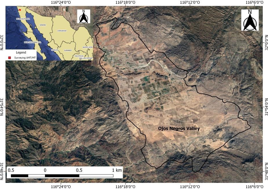
Figure 1. Location of Ojos Negros valley.

Geological and Hydrogeological background

The valley is surrounded by extrusive and intrusive rocks, which form outcrops on the margins and interior hills. Gneiss and schist rocks come from basic and pelitic rocks subjected to intense regional metamorphism due to plutonic thermal events (Gastil et al., 1975). The study area comprises a graben formed by tension forces between two bounding faults and the fall of a block. Weege (1976) describes the main structural features of the valley. The west side has a near-vertical slip fault, so-called the Ojos Negros fault, oriented N20°W with a 350 m high escarpment. The second structural feature, the San Miguel fault system, is located in the northeast part of the valley and has an orientation of N60°W. The North part changes its orientation to N80°W until it meets the Ojos Negros fault. These two geological features limit the graben and generate the topographic depression from the Ojos Negros valley (Weege, 1976). Figure 2 shows the geological map of the study area. The Ojos Negros aquifer belongs to Hydrogeological Region 1 (CONAGUA, 2020). Previous geological and geophysical surveys established that the aquifer is unconfined, heterogeneous, and anisotropic, with local semi-confined conditions due to clay sediments (CONAGUA, 2020).

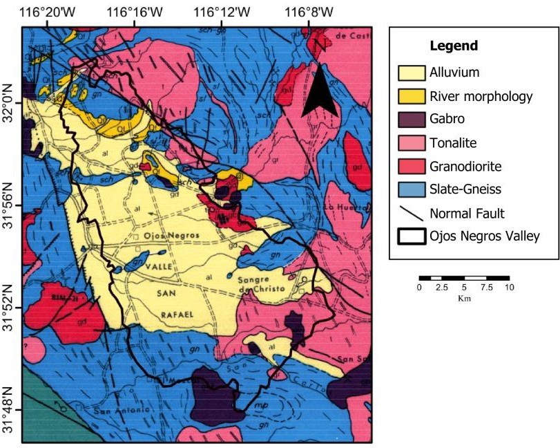
Figure 2. Geological map of the survey area (modified by Gastil et al., 1975).

Field survey

During September and November of 2019, a field campaign was carried out on the east side of the Ojos Negros valley to acquire a total of 32 audiomagnetotelluric soundings (Figure 3). The distribution of the soundings was in two profiles: eighteen (18) and fourteen (14) soundings define a north-south and a west-east profile, respectively. The separation of each station is 150 meters. We measured the variations of the horizontal components of the electric and magnetic fields. Some of the soundings were recorded with ADU-07e devices from Metronix Ltd, whereas the rest of the stations were acquired with a STRATAGEM device from Emi-Geometrics Ltd.

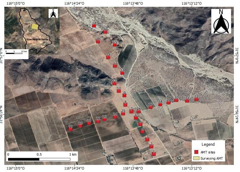
Figure 3. Location of the survey area. AMT soundings are marked with red squares.

1D inversion

For this work, we applied the one-dimensional (1D) inversion methods of Occam (Constable et al., 1987) and Marquardt (1963). We did different modeling tests to choose the best initial model that fits the data to ensure optimal parameterization for all stations. The Occam inversion was performed at each station using an initial homogeneous model of 100 Ωm and 25 layers, with logarithmically equidistant layer thickness. The thickness of the first layer is 5 m, and the depth of the last layer is 3500 m. From the Occam 1D inversion models, we derived the initial model for Marquardt inversion because this technique highly depends on the initial model. A three-layer model is sufficient for almost all stations to fit the observed data. Some of the stations yield a two-layer model.

We analyzed the model uncertainty for a better interpretation. We used two different methods. The first one employs a deterministic Monte Carlo scheme to estimate equivalent models (Spies and Frischknecht, 1991). Thus, when the equivalent models show high variability within a model parameter, we can conclude that it is not well resolved. In the second method, we estimate the parameter importances obtained by transforming the normalized singular values of the Jacobian matrix into the model parameter space (Menke, 1984). Thus, an importance value close to one indicates that the model parameter is well resolved (Ruiz-Aguilar et al., 2018).

Figure 4 illustrates the 1D Occam and Marquardt inversion models obtained at soundings ON03 and ON16. At the sounding ON03, the first conductive layer extends down to 10 m, with a resistivity of 30 Ωm. A second layer has resistivities from 90 to 100 Ωm and extends from 10 to 90 m. The third layer shows resistivities greater than 500 Ωm. For sounding ON16, the shallowest layer has a low resistivity (20 Ωm) and extends down to 10 m. The second layer is located between depths of 10 and 200 m, with a resistivity of 80 Ωm. The stratigraphically deepest layer extends from 200 m with a high resistivity of 1000 Ωm. In addition, the model parameters related to the second and third layers are well resolved, which is visible by the slight variation of the equivalent models, and the importances of such parameters are close to 1. In contrast, the resistivity of the first layer is moderately resolved. The importances range from 0.40 to 0.45, and the equivalent models significantly vary.

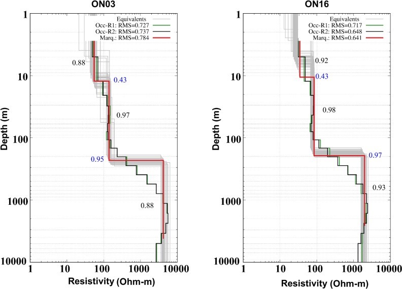
Figure 4. Examples of 1D models were obtained by applying Occam-1R/2R (green and black) and Marquardt (red) inversion techniques corresponding to soundings ON03 and ON16. Equivalent models (gray) are also shown. Parameter importances are marked in black for resistivities and in blue for depths.

3D inversion

We applied the 3D inversion scheme implemented in ModEM software developed by Egbert and Kelbert (2014). In addition, we employed the 3D-Grid software created by Naser Meqbel (Meqbel, 2009). Figure 5 shows the 3D model mesh consisting of 41 x 36 x 65 cells in the X, Y, and Z directions.. The cells size of the X and Y directions is 75 x 75 m sided within the data coverage. In the vertical (Z direction), the thickness of the first layer is 1 m, and the subsequent layers are incremented by a factor of 1.2. Topography was not taken into account because the terrain slopes were not abrupt.

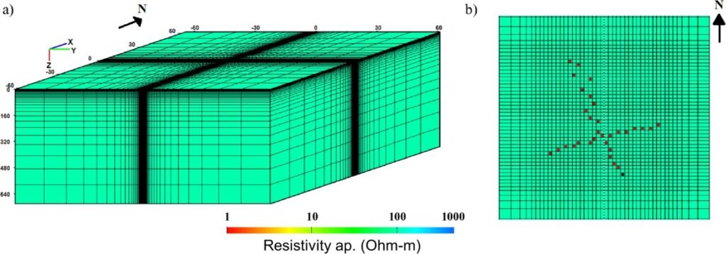
Figure 5. 3D domain used for the inversion (a). Horizontal view of the 3D model domain, where the AMT soundings are displayed by red squares (b).

The 3D inversion was carried out for the off-diagonal components of the impedance tensor. A starting model of 100 Ωm was used. Data errors were set to 5% of |Z_xy * Z_yx|^(½). The covariance parameter was 0.3 in the horizontal direction and 0.4 in the vertical direction. The final inversion model was obtained after 123 iterations, and the reached RMS (root mean square) value was 6.05. Figure 6 displays four resistivity depth-slices extracted from the preferred 3D inversion model.

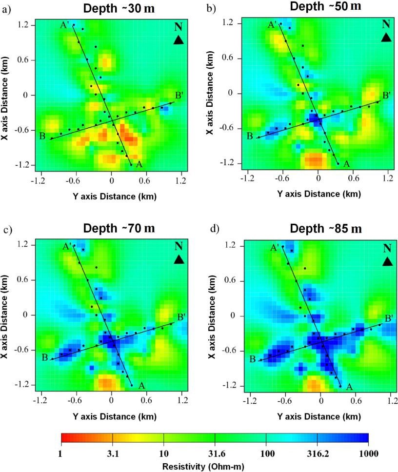
Figure 6. Resistivity slices were extracted from the preferred 3D inversion model.

Discussion

With the different applied inversion techniques in 1D and 3D, it was possible to define the geoelectric units of the study area. One-dimensional models give us a first approximation of the resistivity behavior of the Ojos Negros valley area. For a more detailed interpretation, the 3D inversion model was used.

Profiles A and B were extracted from the preferred 3D inversion model (Fig. 7). In Figure 7, three units are defined; the shallowest unit might be related to the alluvion that outcrops in the survey area, with a thickness of 5-10 m. The second unit, R2, can be correlated to alluvial sediment. This unit is the layer where the aquifer is stored and has a thickness of 65 meters (white dotted line). At the north of profile A, the thickness of unit R2 is greater than beneath the first stations. Therefore, we claim this is an important area because it might store more water. Also, a conductivity body is displayed at the beginning of profile A (C1), enclosed in a black dotted line. This body might be related to the clay lens based on the low resistivity values (1-5 Ωm). In the 1D inversion models, this anomaly appears in the ON04 and ON05 soundings. The anomalies enclosed in the black circles are artifacts of the inversion; sensitive tests corroborate that these anomalies do not exist. The resistivity of the third unit R3 (>500 Ωm) might be related to the crystalline basement, comprised of igneous and metamorphic rocks acting as depth barriers of the overlying aquifer.

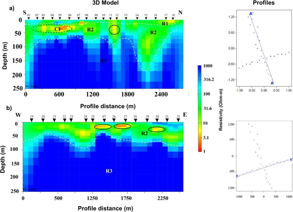
Figure 7. Profiles were extracted from the preferred 3D inverse model.

Conclusions

The information derived from the 32 AMT soundings acquired in Ojos Negros valley allowed the identification of the valley’s hydrogeological units. The 1D and 3D inversion models were helpful to define the hydrogeological units. The low resistivity values observed in the shallowest unit suggest non-saturated sediment conditions. The second one is the most significant unit because it might be related to alluvial sediments (e.g., sands and gravels) that can contain the aquifer. The average thickness of the aquifer is estimated at 65 m, except at the end of profile A where it thickens to 120 m. The third unit shows high resistivities consistent with crystalline basement rocks that seal the aquifer. The advantage of using the 3D inversion was that it helps better define the geometry of the aquifer units.

Acknowledgments

We would like to thank Naser Meqbel for providing us with his 3D-Grid software. The first author acknowledges CONACYT for providing him with a scholarship during his master’s studies.

References

Cassiani, G., Binley, A., and Ferré, T.P., 2006, Unsaturated zone processes, Applied hydrogeophysics: Springer, p. 75-116.

CONAGUA, 2020, Update of the average annual availability of water in the Ojos Negros aquifer (208). Retrieved on February 15, 2022.

Constable, S. C., Parker, R. L., and Constable, CG, 1987, Occam inversion: A practical algorithm for generating smooth models from electromagnetic sounding data: Geophysics, v. 58, no. 3, p 289-300.

Egbert, G. D. and Kelbert, A., 2012, Computational recipes for electromagnetic inverse problems: Geophysical Journal International, v. 189, no. 1, p. 251-267.

Gastil, R., Phillips, R. P., and Allison, E. C., 1975, Reconnaissance geology of the state of Baja California: Geological Society of America, v.140.

Marquardt, D. W., 1963, An algorithm for least-squares estimation of nonlinear parameters: Journal of the Society for Industrial and Applied Mathematics, v. 11, no. 2, p. 431-441.

Menke. W., 1984, Geophysical data analysis: discrete inverse theory, Academic Press.

Meqbel, N. (2009). The electrical conductivity structure of the Dead Sea Basin derived from 2D and 3D inversion of magnetotelluric data. PhD thesis, Freie Universit¨at Berlin.

Ruiz-Aguilar, D., B. Tezkan, and C. Arango-Galván., 2018. Exploration of the aquifer of San Felipe’s geothermal area (Mexico) by Spatially Constrained Inversion of Transient Electromagnetic data: Journal of Environmental and Engineering Geophysics,v. 23, no. 2, p. 197-209.

Spies, B. R. and Frischknecht, C. F., 1991, Electromagnetic Sounding, Electromagnetic Methods in Applied Geophysics: Society of Exploration Geophysics, v. 2, no. A, p. 285-426.

Vozzof, K., 1972, The magnetotelluric method in the exploration of sedimentary basins: Geophysics, v. 37, no. 1, p. 98-141.

Weege, B. C., 1976, Geologic map and geologic interpretation of Ojos Negros Valley, Baja California, Master thesis, San Diego State University.

Yogeshwar, P., Tezkan, B. and Haroon, A., 2013, Investigation of the Azraq sedimentary basin, Jordan using integrated geoelectrical and electromagnetic techniques: Near Surface Geophysics, v. 11, no. 1, p. 381-389.

---

Author Bios