
By : Yao Wang 1, Khiem T. Tran 2,and David Horhota 3
1 PhD student, University of Florida, Department of Civil and Coastal Engineering, 365 Weil Hall, P.O. Box 116580, Gainesville, FL, 32611, US, wangyao@ufl.edu;
2 Associate Professor, PhD, University of Florida, Department of Civil and Coastal Engineering, 365 Weil Hall, P.O. Box 116580, Gainesville, FL, 32611, US, email: ttk@ufl.edu;
3 State Geotechnical Materials Engineer, PhD, Florida Department of Transportation, 5007 N.E. 39th Avenue Gainesville, FL 32609, email: david.horhota@dot.state.fl.us;
Published: 07/05/2021
ABSTRACT
Roadway subsidence poses significant risk to the safety of the traveling public. Detection of subsidence attributes such as buried voids is required for remediation to reduce the risk. Thus, we present a 2D ambient noise tomography (2D ANT) method to characterize roadway substructures for void detection and remediation assessment. The method requires recording of vehicle-induced traffic noise using a linear array of geophones placed along a roadway. The cross-correlation function (CCF) is then extracted from traffic noise recordings and inverted to obtain velocity structures. Passing-by vehicles are assumed as moving sources along the receiver array for the forward simulation and inversion of the CCF. To demonstrate the method’s capabilities, it was applied to field noise data collected both pre- and post-grouting for assessment of a repaired sinkhole under US441 highway, Florida, USA. The pre-grouting result shows that the method is capable of resolving the subsurface S-wave velocity (Vs) structure and detecting a buried void. The post-grouting result suggests that the grouting operation was successful, and the void was sufficiently filled.
INTRODUCTION
Roadway subsidence are mostly caused by buried voids (rock dissolution), and thus detection and remediation of the voids are crucial to minimize the risk to the safety of the traveling public. The invasive Cone Penetration Test (CPT) and Standard Penetration Test (SPT) can be used to obtain detailed information of voids such as the vertical size and depth and filling materials. However, these methods are too expensive or time-consuming to be performed densely along the roadway. Therefore, noninvasive geophysical methods are favorably used for void detection, as they can examine subsurface conditions over a larger volume of materials at lower costs.
Active-source seismic methods are often used for detection of voids by using the refraction, reflection, and surface-wave components of wavefields. They have been used to detect concrete and sandstone tunnels (Chen et al., 2016; Wang et al., 2018), abandoned mines (Sloan, 2017), and sinkholes (Tran et al., 2013; Tran and Sperry, 2018). The active-source testing produces high signal-noise-ratio (SNR) data, and high-resolution results can be achieved. However, as they require multiple source impacts to generate active wavefields, the data acquisition time is significant (hours). This leads to negative impacts caused by closing the traffic flow under seismic testing. In addition, the active sources can trigger sinkhole collapses, particularly when enhancing the low frequencies by adding extra power or weight to the source. Thus, there is need for developing passive source tomography methods by taking the advantage of available ambient traffic noise to minimize the traffic disruption and ground perturbation to avoid collapses.
This study developed a 2D ANT method to invert the cross-correlation function of traffic noise for extraction of subsurface Vs structures. Traffic noise is generated by vehicles running over the road surface. Each moving vehicle can be considered as a pressure load that pushes and then releases the elastic stratum. On a road segment, the traffic is a relatively consistent source of ambient noise because vehicles are restricted within a certain speed range. Relevant research has demonstrated that the Green’s function of the surface waves could be approximated from the urban traffic noise, and the approximated Green’s function can be used to determine the physical properties of the soil and bedrock beneath the roadway (Li et al., 2020; Zhang et al., 2019). However, the required assumption of energy balance at both sides of each receiver pair to retrieve the true Green’s function is not satisfied for cases of individual vehicles passing by the receiver array in only one direction, without vehicles passing in the opposite direction. Therefore, instead of using the approximated Green’s function, we directly invert the cross-correlation function to extract the subsurface structures. The method’s capabilities are evaluated with field noise data collected both pre- and post-grouting at the US441 highway site in Florida, USA, which contains a repaired sinkhole.
METHODOLOGY
The 2D ANT method includes a forward simulation of cross-correlation function, and an adjoint-state inversion for extraction of subsurface material property. Wave propagation is modelled by 2D P-SV elastic wave equations (Levander, 1988; Virieux, 1986). The numerical solution of the P-SV elastic wave equations (Tran and Hiltunen, 2012) is used for simulation of noise fields and Green’s functions required for computing the cross-correlation function during inversion, as discussed in the following sections.
Forward simulation
The cross-correlation function between the two signals and is explicitly given by:
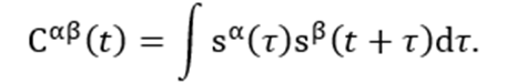
(1)
This explicit formula requires to perform the forward simulation for each source location individually to obtain seismograms sα and sβ. However, utilizing the explicit formula is inadequate for inversion of the cross-correlation function due to a large number of sources with unknown locations of noise fields. To overcome this obstacle, we adopt the implicit simulation method (Sager et al., 2018), which calculates Cαβ with a given source distribution function using reciprocity of Green’s functions at receiver and source locations. Using the Fourier transform, an equivalent form of equation (1) is obtained as:
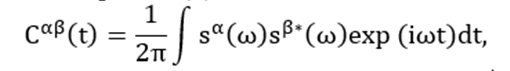
(2)
with the asterisk denotes conjugation. In terms of the Green’s function,

(3)
In the above equation x´, and x´´ are two arbitrary locations in domain Ω. Integrals ∫Ω´ dΩ´ and ∫Ω´´ dΩ´´ denote the integration over domain Ω twice, distinctively.
Next, the cross-correlation function Cαβ (t) is averaged over many realizations as:

(4)
Cαβ (t) is estimated by stacking calculated cross-correlation functions over many time intervals (Bensen et al., 2007). By assuming that the noise is spatially uncorrelated, we therefore approximate with a delta function in space as:

(5)
with the source power-spectrum density (PSD) . For uncorrelated noise sources, equation (6) becomes:

(6)
Using equation 6, we can simulate the cross-correlation function implicitly with a given distribution function of noise source, instead of dealing with noise events individually. The calculation of the cross-correlation function (CCF) between xα and xβ starts with the two forward simulations to obtain Green’s functions G(xα , x, ω) and G(xβ , x, ω) with sources at xα and xβ, respectively. Then, multiply G(xα , x, ω) with the complex conjugate G(xβ , x, ω) and the noise source PSD S(x,ω), and sum over all grid points (integration over space x). Finally, the frequency-domain cross-correlation function is transformed to the time domain. In this study, the PSD is determined from the reverse-time migration of filtered CCF, and S(x,ω) is the same (average value) for all frequencies within the filtering frequency band.
Inversion method
Since the cross-correlation function Cαβ caries the information of Green’s functions with the source at xα and xβ (equation 6), inverting it can retrieve subsurface material property. Considering the misfit between the observed and the synthetic cross-correlation functions,
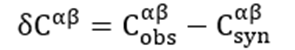
(7)
We use the L2-norm of misfit δCαβ as the objective function,
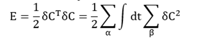
(8)
To calculate the gradient of E with respect to Vs and Vp, we adopt the adjoint-state method derived by Tromp et al., (2010) and Sager et al., (2018). For a given location xα, we can simultaneously backward propagate the difference between the observed and the synthetic cross-correlation functions from all other locations xβ (Tromp et al., 2010). Using stresses of backward-propagated cross-correlation wavefield in the gradient derived for the active-source FWI (Shipp and Singh, 2002), the modified gradient for Lamé parameters λ,μ as:
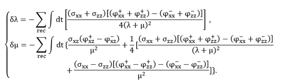
(9)
In equation (9), is the stresses of forward-propagated wavefield and the stresses of backward -propagated cross-correlation wavefield. It is noted that the cross-correlation function Cαβ has a positive lag (t>0 ) and a negative lag (t<0 ), and they need to be calculated separately. Parameters ϕ+ and ϕ– represent the stresses of backward-propagated cross-correlation wavefield for the positive lag and the negative lag, respectively.
Based on the relationships between Vp, Vs, λ,μ ,ρ and density , the gradients with respect to Vp, Vs can be written as:
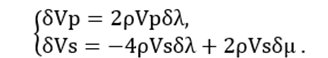
(10)
The steepest descent direction of L2 misfit with respect to elastic velocities is obtained as equation (15), and the model can be updated by:
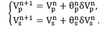
(11)
In equation (11), step lengths θp and θs are computed by a parabolic line search method (Nocedal & Wright, 1999; Sourbier et al., 2009a, 2009b). The model is updated along the steepest descent direction in the first iteration, and then it is updated with the conjugate gradient method to increase the convergence rate. The search direction is calculated following Polak-Ribière method (Klessig and Polak, 1972). Finally, our effort to invert the mass density has been unsuccessful because of its low sensitivity to the cross-correlation dominated by Rayleigh wave energy. Thus, the density is assumed and kept constant during inversion
Field Experiment
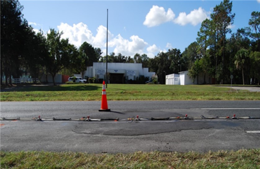
The test site was on US441 Highway, in Marion County, Florida, USA. Experiment was conducted to assess a roadway segment with a repaired sinkhole (Figure 1). The sinkhole caused excessive localized surface settlements in the roadway in 2011, and the roadway was remediated by compaction of filled sand and gravels. However, the subsidence had continued, suggesting that the void was not completely filled (Tran and Justin 2018). After further evaluation, subsurface grouting was selected to remediate the roadway substructure. The 2D ANT method was applied to this site to image the pre-grouting void and assess the post-grouting subsurface. Traffic noise (passive seismic) data sets were acquired along roadway on top of the repaired sinkhole in 2016 (pre-grouting) and 2021 (post-grouting). Data were recorded using a land-streamer of twenty-four 4.5 Hz vertical geophones at 1.5 m spacing for a receiver spread of 34.5 m. The repaired sinkhole is approximately 20 m away from the first receiver.
Pre-grouting data
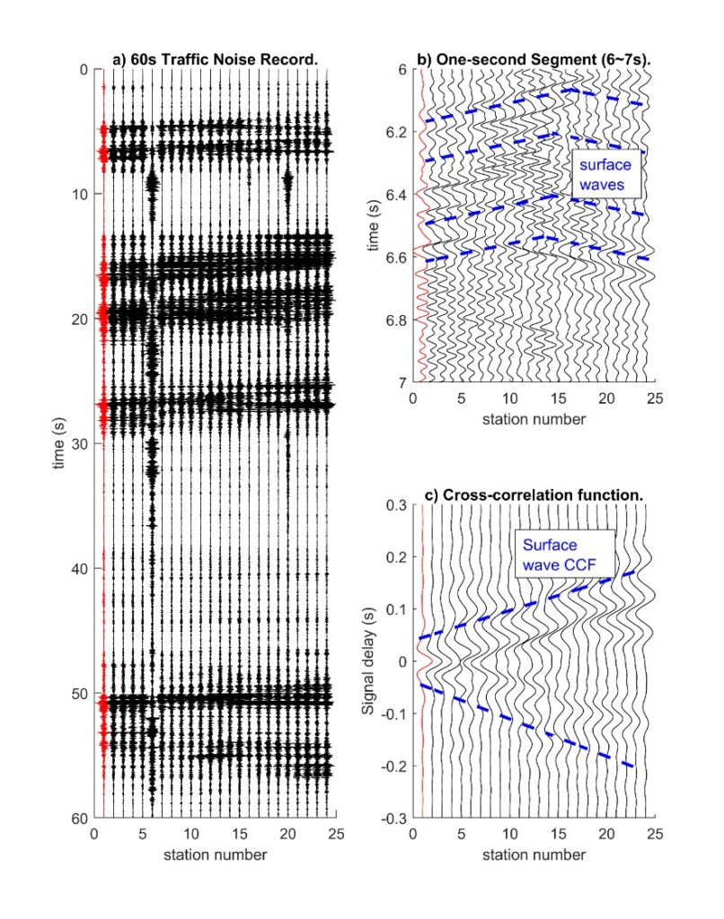
The pre-grouting traffic noise data were collected for five records of one-minute each. A sample record of traffic noises is displayed in Figure 2a, showing strong noise signals of passing-by vehicles between 5~8s, 15~30s, and 48~55s. For this record, most of vehicles passed by in the direction from receiver 24 to receiver 1 (right to left).
The noise data are filtered to preserve the low frequencies (0-25 Hz), and Figure 2b is an example of a segment (6s to 7s) of the traffic noise record. A series of surface wave events (blue dash lines) were induced by passing-by vehicles acting as (internal) sources within the geophone spread, suggesting that a vehicle is a moving active-source and traffic noises are indeed dominated by surface (Rayleigh) waves.
The record was divided into 0.3-second segments. The segment length of 0.3-second was selected, as it is long enough for wavefields to propagate through the entire geophone spread of 34.5 m. A longer segment can also be used, but it potentially leads to cross-correlate wave events from multiple sources (source correlation issue). The cross-correlation function was calculated for each segment and stacked together as shown in Figure 2c. As highlighted with blue dash lines, Rayleigh waves are evident and have a consistent pattern of propagation in the retrieved cross-correlation function.
The source signature and distribution are important for inversion of the cross-correlation functions. As the source spatial distribution of traffic noises is on the road surface and close to the test location, we estimate the source signature and the source power-spectrum density (PSD) only for surface-based sources from the field data and keep them constant during inversion. The source signatures used for forward simulation were estimated from the field noise autocorrelation at reference stations.
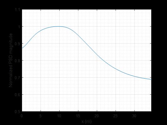
The PSD was estimated by the time-reverse imaging method (Artman et al., 2010) and shown Figure 3a for the source distribution along the ground surface (no embedded source for traffic noise). It shows the comparable source energy along the test line with the largest energy at distance of 10 m. This PSD function is used for simulation of the estimated cross-correlations for inversion.
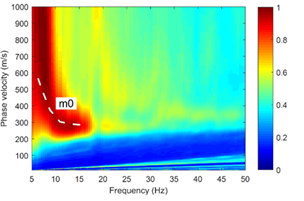
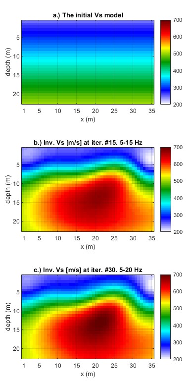
The initial Vs model was established via a dispersion analysis of passive-source surface waves (noise data). The dispersion spectrum image (Figure 3b) is created following the method developed by Park et al. (2004). Rayleigh wave phase velocity ( ) is increasing from 250 m/s to 500 m/s as the frequency decreasing from 15 Hz to 5 Hz, which implies that Vs profile generally increases with depth. The initial Vs model (Figure 4a) is set to be lateral homogeneous with values increasing linearly with depth from 250 m/s to 500 m/s. The initial Vp model is created from the initial Vs model and a characteristic Poisson’s ratio of 1/3.
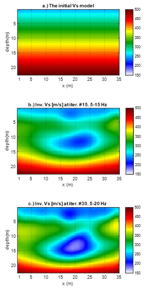
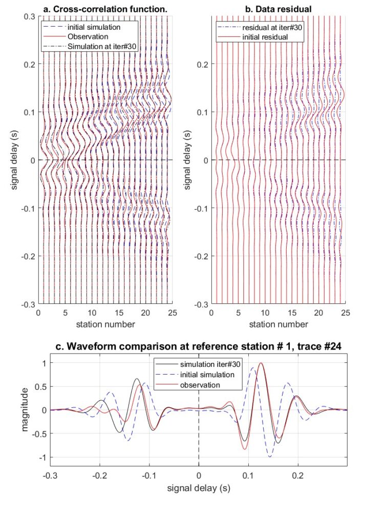
As the consistent cross-correlation signals are available at 5 Hz to 20 Hz, two inversion runs were conducted with frequency bandwidths of 5-15 Hz and 5-20 Hz. The first run started with the lower frequency bandwidth on the initial model (Figure 4a), and the second run continued on the first run result as the input model. Each run stopped at a preset number of iterations (15), and it took about one hour on a desktop computer (8 cores of 3.7 GHz processor and 64 GB RAM) for both runs. The waveform comparison of the observed and simulated cross-correlation functions is shown Figure 5a. The red curves are the observed cross-correlation function of field traffic noise at 5-20 Hz. The blue and black dash curves are the initial and the final simulated cross-correlation functions, respectively. At large-offset channels (16 to 24), the improvement of data fitting during
inversion is evident. The arrival time of the initial simulation is earlier than that of the observation, suggesting the initial model is stiffer than the true subsurface profile. The misfit between the observation and the simulation is minimized during inversion. The residuals (Figure 5b) decreased from the first to final simulations. The remaining residuals are mostly due to noise in the cross- correlation and the potential error in the source estimation. Again, the waveform match improved during inversion.
The inverted Vs profiles of the two runs are shown in Figure 4. The final result of the second run (Figure 4c) clearly shows a low-velocity anomaly at 12 m depth. The anomaly center is at distance x= 20 m, which is the same location of the repaired sinkhole. The inverted Vs at the anomaly center is about 150 m/s, which is lower than the values of the surrounding area (>300 m/s), suggesting that the void was not completely filled and compacted. This was supported by the subsequent subsidence after the pre-grouting testing.
It is noted that the maximum change of Vp values during inversion is only less than 20 % from the initial model and the anomaly is not imaged in the Vp profile, and thus it is not shown herein. This is due to P-wave wavelengths of analyzed frequencies (<20 Hz) is much larger than the anomaly size.
Post-grouting data
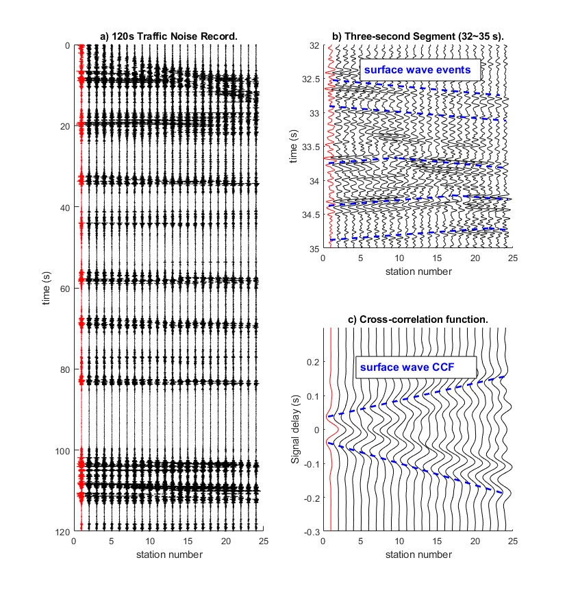
After grouting, traffic noise data were acquired at the US441 site again in January 2021. The acquisition system for the post-grouting data was the same as that of the pre-grouting data. The land-streamer of 24 vertical 4.5Hz geophones at 1.5 m spacing was placed along the roadway on top of the grout. Traffic noise from passing-by vehicles were collected for 10 records of two minutes (120 s) each. With the similar data processing steps of the pre-grouting data, the cross-correlation functions were retrieved from the traffic noise records. Figure 6a displays a 120 s record of the traffic noise after low-pass (< 25 Hz) filtering. It clearly shows noises induced by several passing-by vehicles.
One recorded vehicle event is shown by Figure 6b. In this 3-second record, a vehicle ran through receivers 1 to 24, and generated several surface waves events (highlighted with blue dash lines in Figure 6b). The filtered noise record is then divided into segments of 0.3 s, cross-correlated, and stacked to generate the cross-correlation functions (Figure 6c). The surface wave events (blue dash lines) are evident in the cross-correlation function. The apparent velocity of the surface waves in the cross-correlation function is approximately 250 m/s.
The same initial model as that of the pre-grouting data inversion is used. The initial Vs is linearly increasing from 250 m/s to 500 m/s from the ground surface to 22.5 m depth (Figure 7a). Vp is twice Vs, and the density is set to 1800 kg/m3. Two inversion runs were conducted with frequency bands of 5~15 Hz and 5~20 Hz, respectively, and each run lasted 15 iterations.
The results of both runs are displayed in Figure 7. The final result (Figure 7c) reveals a high-velocity zone with Vs ~700 m/s at distance of 20 m, which is the same location of grouting. This high-velocity zone represents the grouting material and densified soil around the grouting volume. No evident low-velocity zone at the void location (white curve) exists in the inversion result; suggesting that the grouting operation was successful, and the void was sufficiently filled.
CONCLUSIONS
We present a 2D ambient noise tomography (2D ANT) method for assessment of roadway substructure. The cross-correlation function of traffic noise recordings is inverted directly to obtain subsurface Vs profile. Applied on field experimental data, the method demonstrates the great capability in imaging buried high- and low-velocity anomalies. The field experimental result shows that it successfully detects a low-velocity anomaly before grouting and a high-velocity anomaly after grouting. Based on the field result of noise recordings with the minimum disruption of the traffic flow, the presented 2D ANT method is an effective approach for characterization of roadway substructure and detection of anomalies.
REFERENCES
Chen, J., Zelt, C.A., Jaiswal, P., 2016. Detecting a known near-surface target through application of frequency-dependent traveltime tomography and full-waveform inversion to P-and SH-wave seismic refraction data. Geophysics 82, R1–R17.
lessig, R., Polak, E., 1972. Efficient Implementations of the Polak–Ribière Conjugate Gradient Algorithm. SIAM J. Control 10, 524–549.
Levander, A.R., 1988. Fourth-order finite-difference P-SV seismograms. Geophysics 53, 1425–1436.
Li, Y.E., Zhang, Y., Nilot, E., Ku, T., 2020. Passive seismic methods for shallow and deep bedrock detection in Singapore, in: Fifth International Conference on Engineering Geophysics (ICEG). Society of Exploration Geophysicists, pp. 176–180.
Nocedal, J., Wright, S.J., 1999. Numerical Optimization, Springer Series in Operations Research. Springer-Verlag New York Incorporated.
Park, C., Miller, R., Laflen, D., Neb, C., Ivanov, J., Bennett, B., Huggins, R., 2004. Imaging dispersion curves of passive surface waves, in: SEG Technical Program Expanded Abstracts 2004. Society of Exploration Geophysicists, pp. 1357–1360.
Sager, K., Ermert, L., Boehm, C., Fichtner, A., 2018. Towards full waveform ambient noise inversion. Geophys. J. Int. 212, 566–590.
Shipp, R.M., Singh, S.C., 2002. Two-dimensional full wavefield inversion of wide-aperture marine seismic streamer data. Geophys. J. Int. 151, 325–344.
Sloan, S.D., 2017. Role of depth in anomaly detection using near-surface seismic methods, in: International Conference on Engineering Geophysics, Al Ain, United Arab Emirates, 9-12 October 2017. Society of Exploration Geophysicists, pp. 132–135.
Sourbier, F., Operto, S., Virieux, J., Amestoy, P., L’Excellent, J.-Y., 2009a. FWT2D: A massively parallel program for frequency-domain full-waveform tomography of wide-aperture seismic data—Part 2: Numerical examples and scalability analysis. Comput. Geosci. 35, 496–514.
Sourbier, F., Operto, S., Virieux, J., Amestoy, P., L’Excellent, J.-Y., 2009b. FWT2D: A massively parallel program for frequency-domain full-waveform tomography of wide-aperture seismic data—Part 1: Algorithm. Comput. Geosci. 35, 487–495.
Tran, K.T., Hiltunen, D.R., 2012. Two-dimensional inversion of full waveforms using simulated annealing. J. Geotech. Geoenvironmental Eng. 138, 1075–1090.
Tran, K.T., McVay, M., Faraone, M., Horhota, D., 2013. Sinkhole detection using 2D full seismic waveform tomography. Geophysics 78, R175–R183.
Tran, K.T., Sperry, J., 2018. Application of 2D full-waveform tomography on land-streamer data for assessment of roadway subsidence. Geophysics 83, EN1–EN11.
Tromp, J., Luo, Y., Hanasoge, S., Peter, D., 2010. Noise cross-correlation sensitivity kernels. Geophys. J. Int. 183, 791–819.
Virieux, J., 1986. P-SV wave propagation in heterogeneous media: Velocity-stress finite-difference method. Geophysics 51, 889–901.
Wang, Y., Miller, R.D., Peterie, S.L., Sloan, S.D., Moran, M.L., Cudney, H.H., Smith, J.A., Borisov, D., Modrak, R., Tromp, J., 2018. Tunnel Detection at Yuma Proving Ground, Arizona, USA. PART 1: 2D Full-Waveform Inversion Experiment. Geophysics 84, 1–44.
Zhang, Y., Li, Y.E., Zhang, H., Ku, T., 2019. Near-surface site investigation by seismic interferometry using urban traffic noise in Singapore. Geophysics 84, B169–B180.