
By Edward D. Billington, PG1 and C. Ryan Pastrana, GIT ²
1ESP Associates, Inc., Greensboro, NC
²ESP Associates, Inc., Greensboro, NC
Published 07/02/2021
ABSTRACT
The North Carolina Department of Transportation (NCDOT) has been a strong supporter of near-surface geophysics for over 3 decades. When the author began providing geophysical services to the NCDOT in 2001, there were only two firms under contract specifically for geophysics. Currently, there are 30 firms under contract to the Geotechnical Engineering Unit (GEU) with between 10 and 15 of these providing some level of geophysics, either directly or through subconsultants. Geophysical services are used to provide subsurface information for highway widening, bridge replacement, new highway/bridge construction, and issues that arise with existing highways and bridges. Example services include locating abandoned underground storage tanks (USTs), delineating landfills, characterizing depressions and voids, and mapping depth to rock. This paper shows examples of how the NCDOT utilizes these geophysical services for transportation projects in North Carolina.
INTRODUCTION
The process the NCDOT follows for obtaining geophysical services is through their existing contracts, administered by the GEU in the central office. The NCDOT will send a Request for Proposal (RFP) to a specific firm for a particular project, while trying to balance the workload between contractor firms. Requests for geophysics can be stand-alone or can be part of a larger geotechnical or geoenvironmental scope. The majority of the work is planned in advance, although some “emergency” projects require rapid response.
ABANDONED USTS
Much of the geophysical work done for the NCDOT is to locate abandoned USTs for highway widening projects. A Phase 1 environmental study performed by the GEU GeoEnvironmental group or one of their consultants will identify parcels of concern along a planned highway project, such as existing or former gas stations, dry cleaners, and industrial sites. Many of these may contain known and/or abandoned USTs.
The standard approach for locating USTs is to collect closely spaced electromagnetic induction (EM) data using an EM instrument such as a Geonics EM61 metal detector, followed by ground-penetrating radar (GPR). The EM response is compared to the location of known metallic features to eliminate their response, as appropriate. Remaining EM anomalies are evaluated further using GPR to confirm the presence of suspect USTs and estimate their size and burial depth. Correlation is made between the location of pavement patches, concrete pads, and possible fill or vent pipes. Electromagnetic conduction can be used to trace vent pipes to USTs, as the vents are often separated from the USTs by some distance. A probe rod can be used in soft soils to confirm the presence, size, and depth of USTs.
In 2009, the NCDOT GEU GeoEnvironmental group developed a UST rating chart to provide consistency among firms for reporting purposes. The ratings are shown in the table below and are primarily based on the confidence of the geophysical results in indicating a suspect UST. Known, Probable (higher confidence), and Possible (lower confidence) USTs may need to be excavated and removed in a later phase of the project prior to construction.
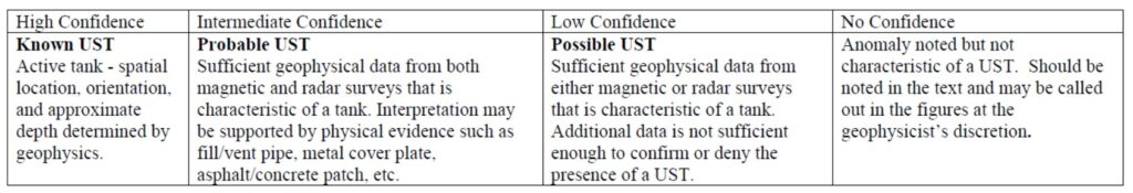
Table 1 . NCDOT UST Confidence Ratings
Example Abandoned UST Study
The planned widening of a highway south of Charlotte, NC required Phase 2 environmental assessments of 8 parcels, including active and former gas stations. The planned work consisted of records research, geophysics to locate known and abandoned USTs, and soil sampling and lab testing to identify areas of contamination.
One vacant parcel had a history of use as a gas station with 4 USTs reportedly removed in 1997. During our November/December 2019 field work, the site was a partially overgrown vacant lot. A slightly elevated concrete slab was present that was probably the former gas station building foundation. Cut-off pipes indicated the location of the former pump islands. The ground in the study area was covered by grass, shrubs, asphalt pavement, and concrete pavement. A sketch map obtained from the North Carolina Department of Environmental Quality (NCDEQ) showed the approximate location of the former USTs. So, the question was: Are there any abandoned USTs on the site that may have predated the known USTs?
We collected EM data using a EM61-MK2 along lines spaced approximately 3 feet apart. The data were collected in differential mode, providing 3 separate time gate responses plus the difference in response between the top coil and the bottom coil (differential response). The differential response removes the response from small, very shallowly buried metallic features, allowing the anomalies from larger, more deeply buried metallic objects such as USTs to be more easily recognized. The location of the former tank pit was heavily overgrown and geophysical data could not be collected in that area. In addition to responses from relic utilities and known site features, the EM61 differential data indicated a UST-sized anomaly at the south end of the site (Figure 1).
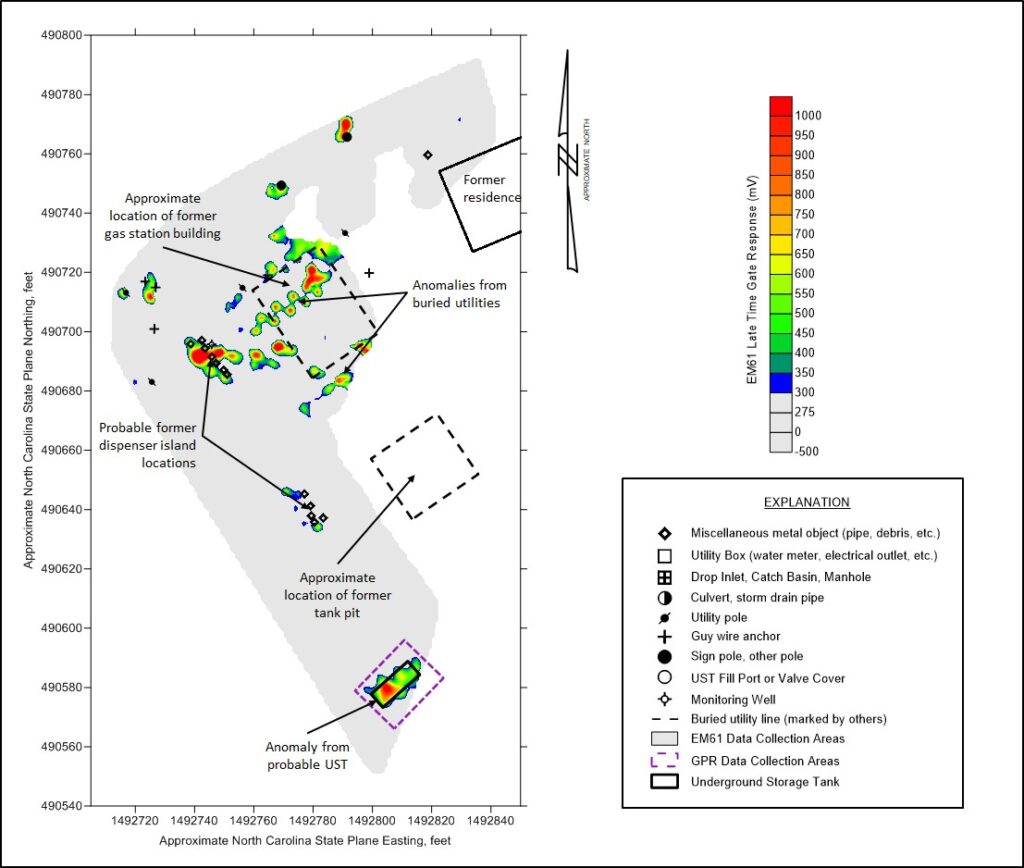
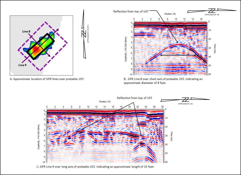
We returned to the site a few weeks later and collected GPR data over the EM61 anomalies using a Sensors and Software Noggin GPR with a 250 MHz antenna. The results indicated a probable UST at the location of the EM61 anomaly at the south end of the site. The GPR data indicated the probable UST was buried approximately 4 feet deep, had a diameter of about 8 feet and a length of about 15 feet, corresponding to a volume between approximately 5000 and 6000 gallons.
DEPRESSIONS AND VOIDS
One of the problems that the NCDOT has to address is the development of depressions and subsurface voids on or adjacent to highways. The majority of these features are caused by failing storm pipes, such as rusting corrugated metal pipes (CMPs). Southeastern NC has some limestone karst features that can affect highways. Also, dewatering due to quarry operations or drought can result in roadway foundation settlement.
Example Void Study
In 2013, a depression was observed and filled by the NCDOT on the outside shoulder of the southbound lanes of US321 near Lincolnton, NC. It was thought that the depression was related to a clogged storm drain in the grassy median between the southbound and northbound lanes, raising concerns for voids existing below the southbound lanes.
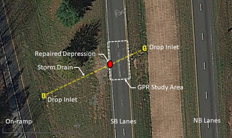
The NCDOT requested that we investigate the site as soon as possible. We mobilized to the site the following day and collected GPR data using a Sensors and Software Noggin GPR with a 250 MHz antenna. The GPR data were collected along lines spaced one foot apart over the southbound lanes in the travel direction. The data were processed using EKKO Project and viewed as 2D cross-sections and as a 3D data set. The results indicated a probable void near the center of the southbound lanes in between the clogged storm drain and the repaired depression on the shoulder.
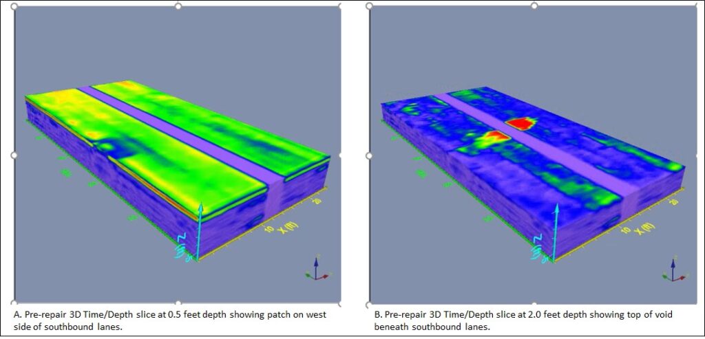
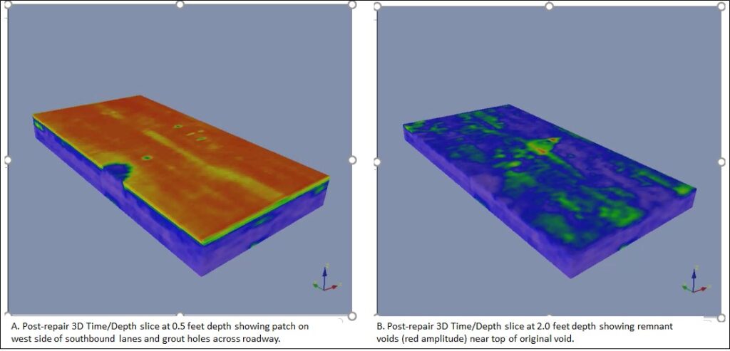
The NCDOT mobilized their grouting crew a few days later, drilled holes in the asphalt where we indicated the location of the void, and injected a cementitious grout into the subsurface void. We had the opportunity to return a year later and repeat the GPR study. The results showed some small remnant voids near the crest of the original void. The results also showed the grout holes from the repair. A Voxler movie of the pre-repair GPR data can be viewed here:
LANDFILLS AND BURIED WASTE
As the population grows and new highways are built, it is inevitable that some new construction will encounter closed municipal and industrial landfills. While landfills provide relatively cheap acreage, construction often requires removal of the waste from the planned highway footprint. Lateral and vertical delineation of the landfill using geophysical and intrusive methods allows waste volumes to be estimated for highway alternatives and construction costs.
Example Landfill Study
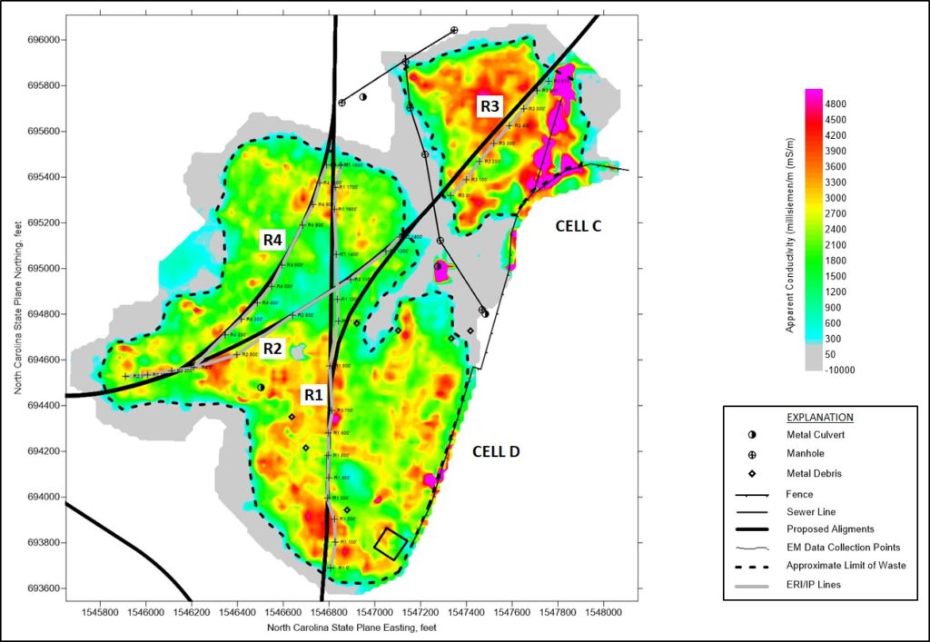
In 2018, the NCDOT began studying alternatives for a new parkway in Rowan County, NC. Some of the proposed alignments passed through a closed municipal landfill. The landfill was reported to have a soil cap with a mix of grass and tree/shrub cover. The closed cells in the study area (Cells C and D) covered an area of approximately 55 acres. The NCDOT asked that we conduct a geophysical study to delineate the limits of the landfill and estimate volumes.
The work consisted of records research, EM data collection, electrical resistivity imaging, and induced potential. The EM data were collected using a Geophex GEM-2 multi-frequency device operated at 5 different frequencies (450Hz, 1530Hz, 5310Hz, 18330Hz, and 63030Hz). The EM lines were spaced approximately 100 feet apart in two orthogonal directions and required clearing for access. A differential GPS (DGPS) was used to provide sub-meter locations of the data as it was collected. The 5310 Hz GEM-2 conductivity correlated well with known limits of the landfill and was used to delineate the lateral extents of Cells C and D.
Following the EM study, we collected Electrical Resistivity Imaging/Induced Potential (ERI/IP) data using a Supersting R8 with 56 electrodes and operated in the dipole-dipole array mode using the roll-along method. Initial tests using an electrode spacing of 20 feet showed high errors and a lack of a significant IP response from the waste. We reduced the electrode spacing to 10 feet for an array length of 550 feet. The results with the shorter array indicated less error than the initial tests but still with a lack of a significant IP response from the waste.
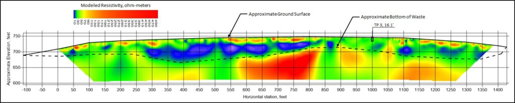
The ERI models produced using EarthImager 2D indicated an approximate thickness of the conductive waste of up to 75 feet. However, since it has been our experience that ERI models overestimate the thickness of municipal waste, we usually rely on the IP response, correlated with test pits or borings. In this case, the IP response was unreliable and tests pits excavated prior to the ERI/IP work did not reach the bottom of the waste.
The volume of the waste was calculated by creating surfaces of the ground surface topography and the approximate bottom of the waste, then calculating the difference for each alignment. The results indicated a minimum of 600,000 cubic yards (cy) of waste and a maximum of 950,000 cy of waste for the various alignments. Although there was concern about the estimated volumes of the waste, the parties agreed that the difference between the estimated and actual volumes was relatively the same for each alignment and the results could be used for helping to select an alignment.
DEPTH TO ROCK
The NCDOT typically uses borings spaced 100 feet apart to develop approximate top of weathered rock and top of competent rock profiles. In some cases, there is insufficient access for a drill rig and the NCDOT supplements their investigations with geophysics. Typically, this occurs in the mountains where the shoulders are very narrow and the adjacent slopes are very steep.
Example Depth to Rock Study
The NCDOT contacted us to provide subsurface information on depth to rock along a planned retaining wall alignment in Ashe County, NC as part of a bridge replacement project. Borings had been drilled by the NCDOT along the existing roadway but these were approximately 30 to 40 feet upslope from the planned retaining wall. The existing slope was too steep for drilling rig access.
ESP collected compressional wave seismic refraction data on 6 lines: Line 1 was located along-slope following the planned retaining wall alignment and 5 lines were oriented downslope starting at the edge of existing pavement. The downslope lines started at or near existing borings for correlation. The refraction data were collected using a 24-channel Geode seismograph, 8 Hz geophones, and a sledgehammer/plate source. Four 115-foot long arrays using 24 geophones were employed for Line 1. Due to the short length of the slope, only 9 to 10 geophones were able to be used for the slope lines with array lengths of 40 to 45 feet. Wooden stakes were placed at 50-foot intervals along Line 1, and at the top, bottom, and significant slope changes on Lines 2, 3, 4, 5, and 6. The steepness of the slope required geophysical personnel to wear safety harnesses and utilize climbing ropes.
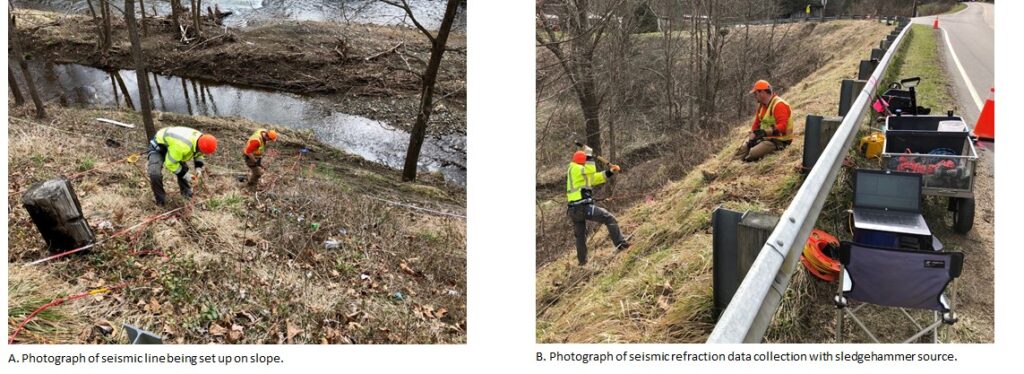
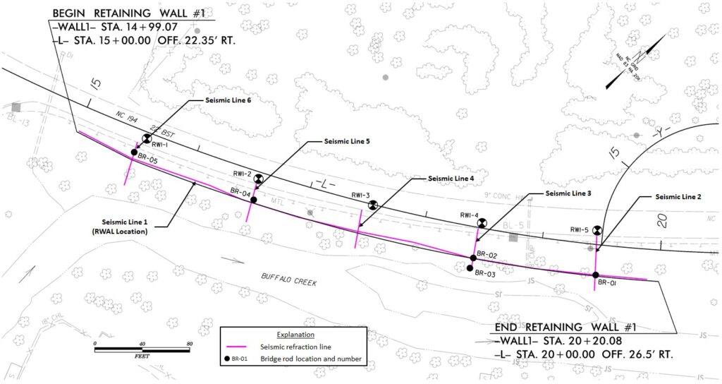
In addition to collecting the seismic data, we drove “bridge rods” at the intersections of Line 1 with Lines 2, 3, 5, and 6. The work consisted of driving 5-foot long, half-inch steel rods with a 16-pound slide hammer approximately vertically down into the ground until refusal. Couplers were used when more than one rod was needed. Notes were recorded as to the relative softness or hardness of the materials that were driven through with the rods, and the depth of refusal. Wooden stakes were placed to mark the location of the rod drives. The locations and elevations of the wooden stakes placed to mark the seismic line locations, rod drives, and existing borings were located utilizing conventional survey equipment.
The seismic data were processed using the program SeisImager, specifically, the modules Pickwin and Plotrefa. The processing steps consisted of assigning geometry, picking the arrival times of refracted energy at each geophone (first breaks), creating an elevation model from the survey point data, then performing a tomographic inversion of the arrival time data to develop a compressional wave velocity model for each line (Figures 10 and 11). The velocities are presented in feet per second (ft/s).
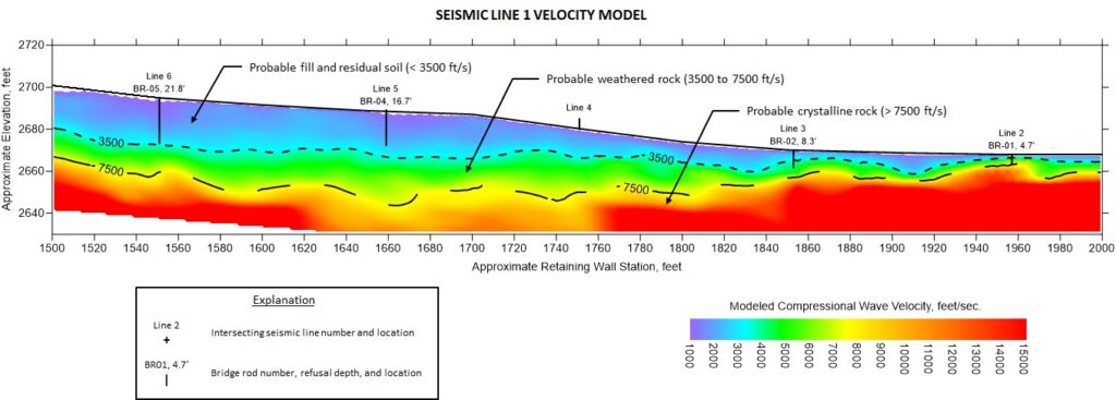
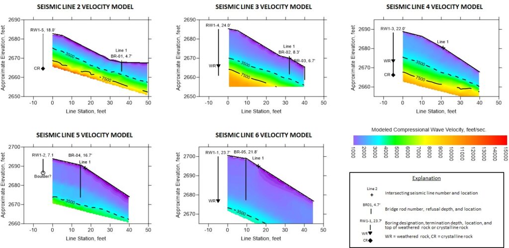
The velocity models were correlated with the rod drives to assess the approximate depth to weathered rock and to crystalline rock. Based on this evaluation, we made the following generalized definitions.
Compressional Wave Velocity (ft/s) | Corresponding Material Type |
| Less 3500 | Fill and Residual Soil |
| 3500 to 7500 | Weathered Rock, WR |
| 7500 or more | Crystalline Rock |
The velocity model for Line 1 indicates that the depth to weathered rock is approximately 20 feet from STA 15+00 to 17+00. After STA 17+00, the depth to weathered rock decreases to 10 feet or less. At rod drive BR-01 on the alluvial bench, the material was soft until almost refusal at 4.7 feet below ground surface (bgs). Based on the seismic velocities, it appears that BR-01 refused on crystalline rock, so there appears to be little to no weathered rock in the vicinity of BR-01; this would be expected for an alluvial stream bank where the stream had previously scoured down to bedrock.
Due to the slope distance from the guard rail to the creek, the length of the arrays for Lines 2 through 6 were too short to obtain sufficient refracted arrivals from crystalline rock, resulting in velocity models that probably do not represent the true velocity structure of the subsurface. Although there is not a satisfactory match between the velocity model for Line 1 and the models for Lines 2 through 6 where they intersect, the models for Lines 2 through 6 do indicate that the depth to weathered rock decreases from STA 15+00 to STA 20+00, supporting the interpretation of Line 1, and they show a reasonable correlation with the adjacent RW1 soil test borings.
On a side note, we extend kudos to the manufacturer of the Geode Seismograph (Geometrics). At one point, the Geode was dropped at the top of the slope at the guard rail, rolled down the slope while bouncing off of rocks on the way down, fell into the stream and floated a few hundred feet downstream before being rescued. The Geode survived intact without any adverse effects. It would have made a great promotional video.
SUMMARY
This paper provides a limited list of example case studies of some of the geophysical methods employed by the NCDOT to help meet their subsurface exploration needs. In addition, there are a number of other geophysical practitioners who have provided a variety of successful geophysical studies for the NCDOT over the years. One of the key factors in the success of geophysics in transportation applications is the availability of boring and test pit data for correlation. The combination of geophysical and intrusive data strengthens the application of both methods.
ACKNOWLEDGEMENTS
The authors thank the NCDOT GEU personnel in the central and regional offices for their support of geophysics over the past 20 years.
Authors Bios
Edward (Ned) D. Billington, PG
Ned Billington is the Geophysical Manager for ESP Associates in Greensboro, North Carolina. He has an undergraduate degree in Geology and Physics from UNC Chapel Hill and a Masters in Geophysical Science from Georgia Tech. After leaving the oil patch in New Orleans, he acquired 30 years of near-surface geophysical experience in North Carolina and other states. His experience includes directing geophysical studies for roadways, bridges, tunnels, dams, reservoirs, hazardous waste, landfills, sinkholes, and voids.
C. Ryan Pastrana, GI
Ryan Pastrana is a Project Geophysicist for ESP Associates and has a BA in Geology from Guilford College. A former Marine, he has 5 years of professional experience on bridge and roadway foundation investigations, Phase 2 hazardous waste investigations, and near-surface geophysical applications.